Dose Rate and Distance: Applying the Inverse Square Law in Radiation Protection

→ Product category: Radiation Measurement Technology

 

If a dose rate of 100 µSv/h is measured at a distance of 1 m from a radioactive point source, an immediate question arises when planning the measurement: What dose rate can be expected at a distance of 2 m? And how large must the distance be for a certain dose-rate value to be expected to fall below a specified level?

For an approximately point-like source, this question can be answered using the inverse square law. If the distance is doubled, the dose rate theoretically decreases to one quarter. At three times the distance, one ninth remains, and at four times the distance, one sixteenth of the original value remains.

This simple law is extremely useful in practical radiation protection. It makes it possible to estimate measuring ranges, plan approaches and assess the potential benefit of a greater working distance before carrying out a measurement. At the same time, it must not be applied uncritically to every radiation source. Extended sources, shielding, scattered radiation, building structures and the natural radiation background can cause actual measured values to deviate significantly from the ideal calculation.

The inverse square law is therefore a tool for physical estimation and measurement planning – not a substitute for an actual dose-rate measurement and not a sufficient basis on its own for defining radiation protection areas.

Suitable measuring equipment is available from ICS Schneider under Radiation Measurement Technology and specifically under Dose Rate Meters.

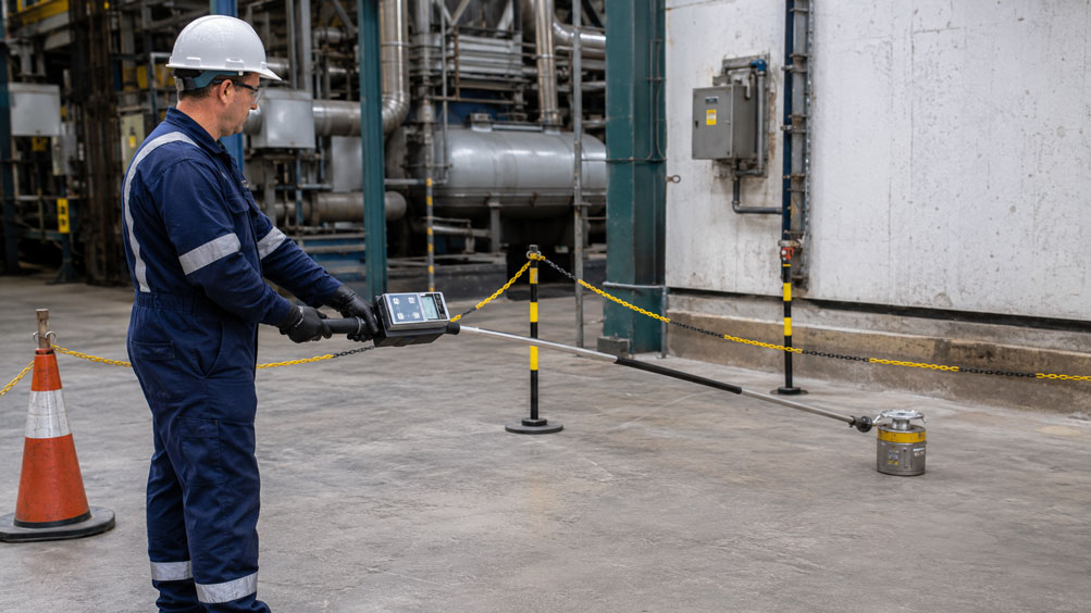
For mobile measurements, for example, the GRAETZ GammaTwin and the GRAETZ X5C plus are available. For higher dose rates or measurements with a greater distance between the operator and the source, the X5C system can also be combined with the GRAETZ Telescopic Probe DE.

Why dose rate decreases with distance

An idealized point radiation source emits radiation spatially in different directions.

As the distance increases, the same emitted radiation is distributed over an increasingly larger area.

The surface area of a sphere is:

A = 4 × π × r²

If the radius is doubled:

r → 2r

the surface area of the sphere becomes:

4 times as large

.

The radiation is therefore distributed over four times the area.

The intensity, or with a suitable radiation geometry also the dose rate, decreases to:

1 / 4

of the original value.

This geometric effect is the basis of the inverse square law

It explains why increasing the distance from an external radiation field can be a particularly effective way of reducing exposure.

In practical radiation protection, three basic influencing factors are therefore often considered together:

• reduce exposure time,
• increase distance,
• use suitable shielding.

How these measures are to be applied in practice must, however, be determined for the specific installation and radiation protection task.

Formula of the inverse square law

For an ideal point source:

Ḣ ∝ 1 / r²

For two different distances, the following equation can therefore be used:

Ḣ₂ = Ḣ₁ × (r₁ / r₂)²

Where:

• Ḣ₁ = dose rate at the first measuring point,
• Ḣ₂ = expected dose rate at the second measuring point,
• r₁ = first distance from the source,
• r₂ = second distance from the source.

Important

Both distance values must be entered using the same unit.

For example:

0.5 m and 2 m

or:

50 cm and 200 cm

.

The unit of the dose rate remains unchanged in this ratio calculation.

Thus:

100 µSv/h

will again produce a result in:

µSv/h

.

Typical distance factors in direct comparison

New distance	Dose rate compared with initial value	Example with an initial value of 100 µSv/h
1 × distance	1	100 µSv/h
1.5 × distance	1 / 2.25	approx. 44.4 µSv/h
2 × distance	1 / 4	25 µSv/h
3 × distance	1 / 9	approx. 11.1 µSv/h
4 × distance	1 / 16	6.25 µSv/h
5 × distance	1 / 25	4 µSv/h
10 × distance	1 / 100	1 µSv/h

The table illustrates the significant influence of distance.

However, the reverse direction is equally important

If the distance is halved:

r₂ = 0.5 × r₁

the theoretical dose rate increases by a factor of:

4

.

Approaching an unknown source can therefore result in much greater changes than a linear assessment would suggest.

Calculation example: dose rate at a greater distance

At a distance of:

r₁ = 1 m

a dose rate of:

Ḣ₁ = 80 µSv/h

is measured.

The theoretical dose rate at:

r₂ = 2.5 m

is to be determined.

Calculation

Ḣ₂ = 80 µSv/h × (1 m / 2.5 m)²

Ḣ₂ = 80 µSv/h × 0.16

Ḣ₂ = 12.8 µSv/h

Result

Under idealized point-source conditions, approximately:

12.8 µSv/h

would be expected at a distance of 2.5 m.

This value is a calculated expectation. The actual value must be verified at the intended measuring point.

Calculate the required distance for a desired dose rate

The inverse square law can also be rearranged to calculate the required distance.

Starting from:

Ḣ₂ = Ḣ₁ × (r₁ / r₂)²

the result is:

r₂ = r₁ × √(Ḣ₁ / Ḣ₂)

Example

The measured value is:

80 µSv/h at 1 m

For measurement planning purposes, the distance at which only:

10 µSv/h

would theoretically be expected is to be estimated.

Therefore:

r₂ = 1 m × √(80 / 10)

r₂ = 1 m × √8

r₂ ≈ 2.83 m

Under ideal point-source conditions, approximately:

2.8 m

would therefore be required.

This value is not an automatically valid safety limit

It can be used to prepare a measurement.

However, a real area must not be released or assessed as safe solely on the basis of this calculation.

The actual dose rate, radiation geometry, shielding and operational or regulatory radiation protection requirements must be taken into account.

From dose rate to accumulated dose

Dose rate describes dose per unit of time.

For an approximately constant dose rate, the following simplified relationship applies:

H = Ḣ × t

Where:

• H = dose,
• Ḣ = dose rate,
• t = exposure time.

Example

At:

Ḣ = 20 µSv/h

and an exposure time of:

15 min = 0.25 h

the calculated dose is:

H = 20 µSv/h × 0.25 h

H = 5 µSv

Doubling the distance can therefore also significantly reduce the dose received during an activity

If a point source behaves ideally and the working time remains unchanged, doubling the distance reduces the dose rate and therefore also the corresponding dose contribution to approximately one quarter.

In practice, however, the distance and radiation field can change during an activity. In this case, the actual time-dependent dose rate must be integrated or suitable dosimetry must be used.

When can a source be considered a point source?

The inverse square law assumes a point source.

However, every real source has spatial dimensions.

The point-source approximation becomes increasingly accurate as the dimensions of the radiation source become smaller relative to the measuring distance.

Typical situations that may approximately behave like a point source include

• small sealed radioactive sources at a sufficiently large distance,
• small sources inside a compact source container,
• small X-ray focal spots at a suitable distance and with suitable radiation geometry.

The following should not be treated as point sources without further assessment

• large contaminated surfaces,
• long pipelines with radioactive deposits,
• large vessels containing radioactive material,
• extended bulk materials,
• large activated components,
• several spatially separated individual sources.

The closer the detector is to an extended source, the more strongly the actual distance dependence can deviate from the ideal 1/r² behavior.

From which point is the distance measured?

For a reliable calculation, it must be clear what is meant by the distance:

r

.

On the source side

for an ideal point source, the distance is measured from the location of the radiation source.

With a sealed source, this point may be located inside:

• a capsule,
• a source holder,
• a shielding container.

The distance from the outer surface of the housing is therefore not necessarily identical to the physically relevant distance from the center of the source.

On the measuring instrument side

the position of the sensitive detector is decisive.

With some instruments, the actual detector is located several centimeters behind the surface of the housing.

At short measuring distances, this difference can already have a significant influence on the calculation.

If the manufacturer specifies a reference point or detector marking, it should be used for reproducible distance measurements.

Why radiation background must be taken into account

A dose rate meter also displays a natural or local background value when the source being investigated is absent.

At high dose rates, this contribution is often negligible.

At low dose rates, however, it can become relevant.

The inverse square law applies to the contribution from the source

In simplified form:

Ḣsource = Ḣmeasured − Ḣbackground

When calculating the value at another distance, the source contribution should therefore first be used:

Ḣsource,2 = Ḣsource,1 × (r₁ / r₂)²

The background can then be added again:

Ḣtotal,2 = Ḣsource,2 + Ḣbackground

Why this is important

As the distance increases, the contribution from the source becomes increasingly smaller.

The natural background, however, does not decrease according to the distance law relative to the source being investigated.

The total measured value therefore approaches the local background as the distance increases.

The measurement curve may therefore appear to “flatten out”.

Do not confuse distance with shielding

The inverse square law initially describes a geometric effect.

Shielding, on the other hand, reduces radiation through interaction with matter.

In simplified form, both effects can occur simultaneously:

Dose rate = distance effect × shielding effect

A wall between the source and measuring point therefore changes the situation

The dose rate is no longer determined solely by:

1 / r²

.

The result is additionally influenced by factors such as:

• material,
• thickness,
• photon energy,
• geometry,
• scattered radiation.

A measured value behind shielding should therefore not simply be extrapolated back to an unshielded measuring point.

Influence of scattered radiation and the environment

The ideal inverse square law considers a source in a simplified geometry.

In real installations, however, photons can interact with:

• walls,
• floors,
• ceilings,
• machine components,
• pipelines,
• vessels,
• shielding.

They can be scattered by these structures.

Radiation can therefore reach the measuring point via additional paths

The measured value then consists, in simplified terms, of:

direct radiation + scattered radiation + background

Only the direct contribution from the source follows the ideal distance law approximately under suitable conditions.

Typical consequence

At a greater distance, the measured dose rate may be higher than predicted by the pure point-source calculation.

This does not necessarily mean that the measurement is incorrect.

The environment can contribute additional radiation.

Why the law deviates for extended sources

With an extended source, the photons reaching the detector do not originate from a single point.

Each part of the source is at a different distance from the detector.

The total value results from the superposition of many individual contributions.

Example: large contaminated surface

When the detector is moved away from a large surface, the distance to each individual surface element increases.

At the same time, however, the detector may “see” a larger proportion of the entire surface.

The dose rate therefore does not necessarily decrease according to:

1 / r²

.

As the distance increases

a spatially limited source may increasingly appear point-like.

The point-source approximation may then become more accurate again.

However, there is no universally applicable fixed distance independent of source size and geometry.

Directional and shielded radiation fields

Not every radiation source emits isotropically in all directions.

A source container, for example, may have only a defined radiation exit opening.

In X-ray systems, radiation is also typically limited to a specific area.

The dose rate then additionally depends on direction

A measured value at:

1 m in front of the radiation exit opening

can differ significantly from a measured value at:

1 m to the side of the source container

.

Distance information alone is therefore not sufficient.

For reproducible measurements, the following should be documented:

• measuring direction,
• measuring height,
• distance,
• detector orientation,
• operating condition of the source.

Correctly select the measuring range of the dose rate meter

When planning a measurement, it is not sufficient to estimate only the dose rate that may be expected for the person carrying out the measurement.

The measuring range of the instrument must also be taken into account.

Example

A measuring instrument has a maximum dose-rate measuring range of:

70 mSv/h

However, a preliminary estimate indicates that the intended measuring point could reach:

150 mSv/h

.

This measuring point would therefore be unsuitable for quantitative measurement using this measuring range.

Useful measurement planning should therefore start, wherever possible, with the highest plausible value

Factors to consider include:

• known measured values at other positions,
• source activity or installation information,
• source geometry,
• shielding,
• possible operating conditions,
• measuring range of the detector.

The measuring instrument should not first be introduced into an unknown high dose-rate field merely to find out whether its measuring range is sufficient.

Distinguish between overload range and measuring range

With radiation measuring instruments, a distinction must be made between different specifications.

Depending on the device, these can include:

• display range,
• measuring range,
• alarm range,
• overload range,
• maximum permissible dose rate.

These specifications do not mean the same thing

A detector may, for example, withstand a very high dose rate without immediate damage even though specified quantitative measurement is no longer possible at that level.

Conversely, a display may be capable of showing a larger numerical range than the specified measuring range of the sensor.

For a reliable measurement, the:

specified measuring range

must therefore be used.

Plan measurements from a safe distance

The inverse square law can be particularly useful for planning a measurement before approaching a source.

Example procedure

1. Collect available information about the source and type of radiation.
2. Document a known dose-rate value and the corresponding measuring distance.
3. Check whether the source geometry is suitable for a point-source approximation.
4. Calculate expected dose rates for greater distances.
5. Check the measuring range of the intended measuring instrument.
6. Begin the measurement from as great a distance as reasonably possible.
7. Measure the dose rate at the actual measuring point.
8. Approach further only within the framework of the defined radiation protection concept.
9. Compare measured values with the calculated expectations.
10. Evaluate deviations caused by geometry, shielding, scattered radiation or background.

The specific procedure must comply with the operational radiation protection requirements and the respective measurement task.

Use telescopic probes to increase distance

At high dose rates, one technically useful option is to spatially separate the detector from the operator.

The detector can be positioned closer to the measuring point while the operator remains at a greater distance.

GRAETZ Telescopic Probe DE

The GRAETZ Telescopic Probe DE offered by ICS Schneider is specifically designed for measuring high dose rates from a greater distance or at difficult-to-access locations.

ICS specifies, among other things:

• measured quantity: ambient dose equivalent rate Ḣ*(10),
• dose-rate measuring range from 1.5 µSv/h to 10 Sv/h,
• continuously extendable stainless-steel telescope up to a total length of 4 m,
• automatic measuring range switching,
• use with instruments from the GRAETZ X5C series.

The physical benefit of the additional distance can be considerable

If, for example, a source behaved as an ideal point source and the operator distance could be increased from:

1 m

to:

4 m

the purely geometric dose-rate factor at the respective position would theoretically be:

(1 / 4)² = 1 / 16

.

The actual exposure naturally depends on the overall geometry, the positions of the detector and operator, and the surrounding environment.

Consider measuring time and statistical fluctuations

Many radiation measuring instruments use counting tubes or other detectors in which individual radiation events occur statistically.

Especially at low dose rates, the displayed value can therefore fluctuate.

Short measuring time

may result in relatively large statistical fluctuations.

Longer measuring time

can improve statistical reliability but at the same time increases the time spent at the measuring point.

These two requirements must be weighed against each other when planning an actual measurement.

Depending on the device, averaging or integration time may be handled automatically.

When comparing several distances

measurement conditions should be kept as comparable as possible:

• same operating condition of the source,
• same detector orientation,
• sufficient stabilization of the measured value,
• defined measuring distance,
• comparable environmental conditions.

Do not confuse dose and dose rate

The terms:

dose

and:

dose rate

describe different quantities.

Dose rate

describes the instantaneous dose per unit of time, for example:

µSv/h

Dose

describes the exposure accumulated over a period of time, for example:

µSv

The inverse square law directly relates to the radiation field or dose rate

The dose actually received additionally depends on how long a person remains in the radiation field.

A high value for a short period and a lower value for a longer period can therefore result in similar total doses.

Distinguish between area dose and personal dose

Area dose quantities are frequently used for measurements within a radiation field.

For gamma and X-ray radiation, the GRAETZ dose-rate meters mentioned here measure, among other things, the:

ambient dose equivalent rate Ḣ*(10)

.

Personal dosimetry uses a different measured quantity

For determining personal dose, for example, the personal dose equivalent:

Hp(10)

is used.

A dose-rate meter used for area measurements therefore does not automatically replace a required personal dosimeter.

The measurement task must be clearly defined before selecting the instrument.

Typical errors in distance measurements

Observation	Possible cause	Recommended check
Doubling the distance does not result in approximately one quarter	source is not sufficiently point-like	check source size relative to measuring distance
Dose rate hardly decreases at large distances	background or scattered radiation contribution becomes dominant	measure background separately
Measured value is higher than calculated	scattered radiation or additional sources present	investigate the environment and source distribution
Measured value is lower than calculated	shielding or self-absorption	check materials between source and detector
Large differences at the same distance	directional radiation field or shielding geometry	document and compare measuring direction
Calculation and measurement agree poorly close to the source	source dimensions and detector geometry are relevant	use a greater distance and evaluate the geometry
Calculated distance is systematically incorrect	incorrect reference point for distance	check source center and detector reference point
Measured value fluctuates strongly	statistical fluctuations at low count rate	use a suitable integration time or averaging
Instrument no longer shows a plausible increase when approaching the source	measuring range exceeded or detector overload possible	check measuring range and overload behavior
Dose-rate meter and personal dosimeter show different values	different dose quantities and geometries	compare H*(10), Hp(10) and intended instrument use

Practical example: moving the measuring point from 0.5 m to 2 m

At a small sealed source, the following is measured at:

r₁ = 0.5 m

:

Ḣ₁ = 160 µSv/h

The theoretical dose rate at:

r₂ = 2 m

is to be determined.

Distance ratio

r₂ / r₁ = 2 / 0.5 = 4

The distance is therefore increased by a factor of four.

Dose-rate factor

1 / 4² = 1 / 16

Calculation

Ḣ₂ = 160 µSv/h / 16

Ḣ₂ = 10 µSv/h

Result

Under ideal point-source conditions, increasing the distance from 0.5 m to 2 m would reduce the dose rate from:

160 µSv/h

to approximately:

10 µSv/h

.

The actual value must then be verified by measurement.

Practical example: estimating a minimum distance

A known measured value is:

300 µSv/h at a distance of 1 m

For planning a more distant measuring point, the distance at which:

25 µSv/h

would theoretically be reached is to be estimated.

Calculation

r₂ = 1 m × √(300 / 25)

r₂ = 1 m × √12

r₂ ≈ 3.46 m

The calculated distance is therefore approximately:

3.5 m

For practical use

This value is suitable as a starting point for measurement planning.

Whether 25 µSv/h or less actually occurs at this point must be determined using a suitable dose-rate meter.

Practical example including background radiation

At a distance of 1 m, the measured value is:

2.1 µSv/h

The local background is:

0.1 µSv/h

Step 1: Determine the contribution from the source

Ḣsource,1 = 2.1 − 0.1

Ḣsource,1 = 2.0 µSv/h

Step 2: Calculate the source contribution at 2 m

Ḣsource,2 = 2.0 × (1 / 2)²

Ḣsource,2 = 0.5 µSv/h

Step 3: Add the background again

Ḣtotal,2 = 0.5 + 0.1

Ḣtotal,2 = 0.6 µSv/h

The expected total measured value is therefore approximately:

0.6 µSv/h

and not simply one quarter of 2.1 µSv/h.

At even greater distances, the influence of the background becomes increasingly important.

Systematically plan a dose-rate measurement

1. Define the measurement task: Distinguish between dose rate, dose, search measurement and area monitoring.
2. Identify the type of radiation: Consider gamma, X-ray, beta, alpha or mixed radiation fields.
3. Define the measured quantity: For example ambient dose equivalent rate Ḣ*(10).
4. Evaluate the source geometry: Distinguish between a point source, extended source or multiple sources.
5. Record known measured values: Document the dose rate and corresponding measuring distance.
6. Determine the background: Particularly important at low dose rates.
7. Apply the distance law only with suitable geometry: Recalculate the source contribution for planned measuring distances.
8. Estimate the highest plausible measured value: Select the measuring range of the instrument accordingly.
9. Check the measuring instrument: Verify measuring range, energy range, measured quantity and overload behavior.
10. Maximize the distance: Within the specified working procedure, begin the measurement from as great a distance as possible.
11. Use a remote or telescopic probe if necessary: Position the detector closer to the measuring point without requiring the operator to be at the same distance.
12. Define the measurement geometry: Document distance, direction, height and detector orientation.
13. Measure the actual value: Do not use the calculation as a substitute for measurement.
14. Evaluate deviations: Consider shielding, scattered radiation, source dimensions and additional sources.
15. Consider exposure time: Evaluate the corresponding dose contribution from dose rate and time.
16. Document the measured values: Record unit, measuring instrument, position, time and operating condition.

Suitable radiation measurement technology at ICS Schneider

GRAETZ GammaTwin

The GRAETZ GammaTwin is a compact dose-rate meter for gamma and X-ray radiation.

ICS Schneider specifies, among other things:

• measured quantity: ambient dose equivalent rate Ḣ*(10),
• ambient dose equivalent H*(10),
• energy-compensated Geiger-Müller tube,
• dose-rate measuring range 0.5 µSv/h … 70 mSv/h,
• dose-rate display range up to 70 mSv/h,
• simultaneous or separate display of dose and dose rate,
• preset dose and dose-rate alarm thresholds.

The instrument is therefore particularly suitable for mobile dose-rate measurements within its specified measuring range.

GRAETZ X5C plus

The GRAETZ X5C plus is an expandable dose-rate measuring system.

ICS Schneider specifies, among other things:

• measurement of gamma and X-ray radiation,
• measured quantity Ḣ*(10),
• energy-compensated Geiger-Müller tube,
• dose-rate measuring range of the basic instrument from 1 µSv/h … 19.99 mSv/h,
• dose-rate and dose display,
• peak and average dose-rate display,
• programmable dose and dose-rate alarm thresholds,
• connection for external probes,
• measuring range extension with suitable probes up to 10 Sv/h.

The ability to connect different probes is particularly useful when the measuring range and measurement geometry need to be adapted to different radiation protection tasks.

GRAETZ Telescopic Probe DE

The GRAETZ Telescopic Probe DE is specifically designed for dose-rate measurements from a greater distance.

Specifications include, among other things:

• dose-rate measuring range 1.5 µSv/h … 10 Sv/h,
• display range up to 10 Sv/h,
• measurement of ambient dose equivalent rate Ḣ*(10),
• continuously extendable telescope up to a total length of 4 m,
• use with the GRAETZ X5C series,
• automatic measuring range switching.

This makes it possible to practically incorporate the physical benefit of greater operator distance into the measurement.

GRAETZ GWL10m for area monitoring

If the task is not only to take an individual measurement but also to monitor an area for elevated gamma or X-ray radiation, the GRAETZ GWL10m is also available.

ICS specifies, among other things:

• dose-rate measuring range 1 µSv/h … 80 mSv/h,
• energy-compensated Geiger-Müller tube,
• several defined dose-rate alarm thresholds,
• visual and audible alarm,
• use for area monitoring.

An overview of further systems is available under Radiation Measurement Technology at ICS Schneider.

Conclusion

The inverse square law is one of the most important simple relationships for planning dose-rate measurements on approximately point-like radiation sources.

Doubling the distance theoretically reduces the dose rate to one quarter

For an ideal point source:

Ḣ₂ = Ḣ₁ × (r₁ / r₂)²

At three times the distance, one ninth remains, and at four times the distance, one sixteenth of the original source contribution remains.

The required distance can also be estimated

Using:

r₂ = r₁ × √(Ḣ₁ / Ḣ₂)

a new theoretical measuring distance can be calculated from a known measured value.

The point-source approximation has clear limitations

Extended sources, multiple sources, shielding, directional radiation fields and scattered radiation can result in significant deviations.

At low dose rates, the background must be taken into account

Only the contribution from the source follows the distance law. As the distance increases, the total measured value therefore approaches the local background.

The measuring range must already be considered during planning

A dose-rate meter must be able to measure the value that may occur at the measuring point within its specified measuring range. Display range, measuring range and overload range must not be confused.

Greater distance can also be used as part of the measurement concept

Telescopic or remote probes make it possible to position the detector at the required location while simultaneously increasing the distance of the operator.

For practical applications

Define the radiation type and measured quantity → evaluate the source geometry → record a known measured value and distance → take the background into account → estimate the expected dose rate using the inverse square law → check the measuring range of the instrument → start the measurement from as great a distance as possible → measure the actual values → consider geometry, shielding and scattered radiation → evaluate dose rate and exposure time together → document measuring points and operating conditions.

FAQ: Dose Rate, Distance and the Inverse Square Law

How does dose rate change with distance?

For an ideal point source, the dose rate decreases inversely proportional to the square of the distance.

What is the formula for the inverse square law?

For two measuring distances, Ḣ₂ = Ḣ₁ × (r₁ / r₂)².

What happens to the dose rate when the distance is doubled?

For an ideal point source, it decreases to one quarter of the original value.

What happens at three times the distance?

The dose rate theoretically decreases to one ninth.

What happens at four times the distance?

The dose rate theoretically decreases to one sixteenth.

What happens if I halve the distance?

For an ideal point source, the dose rate theoretically increases by a factor of four.

Why does the inverse square law apply?

Because the radiation emitted by a point source is distributed over the surface of a sphere as the distance increases, and the area of this sphere increases proportionally to r².

How do I calculate the dose rate at another distance?

Using Ḣ₂ = Ḣ₁ × (r₁ / r₂)².

How do I calculate the required distance for a specific dose rate?

Using r₂ = r₁ × √(Ḣ₁ / Ḣ₂).

If I measure 100 µSv/h at 1 m, how much would it be at 2 m?

Under ideal point-source conditions, approximately 25 µSv/h.

How much would it be at 3 m?

Starting from 100 µSv/h at 1 m, approximately 11.1 µSv/h would theoretically be expected at 3 m.

How much would it be at 10 m?

For an ideal point source, approximately 1 µSv/h would be expected at 10 m if the dose rate is 100 µSv/h at 1 m.

Does the inverse square law apply to every radioactive source?

No. In this simple form, it applies to a point source or a source that is sufficiently small relative to the distance under suitable geometric conditions.

What is a point source?

A point source is an idealized model in which the spatial dimensions of the source are sufficiently small compared with the distance being considered that the radiation appears to originate approximately from a single point.

Does the law apply to a large contaminated surface?

Not without further assessment. An extended surface has a different geometry and can deviate considerably from the 1/r² relationship.

Does the law apply to a large radioactive vessel?

Only approximately if the vessel appears sufficiently small relative to the measuring distance and other influences can be neglected.

Does the distance law apply behind shielding?

The geometric distance effect may still be present, but shielding additionally affects the radiation. The measured value therefore cannot be described solely by 1/r².

Why does the calculation sometimes not match measurements inside a building?

Walls, floors, ceilings and installation components can scatter or shield radiation. This changes the actual radiation field.

What is scattered radiation?

Scattered radiation is produced when radiation interacts with matter and subsequently continues in a different direction.

Does the natural background need to be taken into account?

Yes, particularly at low dose rates. For application of the inverse square law, the source contribution should ideally be considered, meaning the measured value minus the local background.

Why does the measured value approach the background at large distances?

The contribution from the source becomes increasingly smaller as the distance increases, while the local background remains present.

What is dose rate?

Dose rate describes a dose per unit of time and is specified, for example, in µSv/h or mSv/h.

What is the difference between dose and dose rate?

Dose describes accumulated exposure, while dose rate indicates how quickly this dose is accumulated.

How do I calculate a dose from a dose rate?

For a constant dose rate, approximately using H = Ḣ × t.

Does doubling the distance also reduce the dose?

If the source behaves like a point source and the exposure time remains the same, the corresponding dose contribution theoretically also decreases to approximately one quarter.

From where is the distance to the source measured?

Ideally from the effective source point or source center to the relevant reference point of the detector.

Why is the position of the detector important?

The sensitive detector is not located directly at the housing surface in every measuring instrument. At short distances, this difference can have a significant influence on the calculation.

May I calculate a safety limit solely using the inverse square law?

No. The law can be used for estimation and measurement planning. A safety-related assessment must be based on actual measurements and the applicable radiation protection requirements for the specific application.

Why should a measurement preferably begin from a greater distance?

With a point source, the dose rate can increase quadratically as the distance decreases. A greater initial distance therefore reduces the likelihood of unexpectedly entering a significantly higher radiation field.

What must I consider regarding the measuring range?

The expected dose rate must be within the specified measuring range of the instrument being used.

Are display range and measuring range the same?

Not necessarily. An instrument may be able to display values outside its specified quantitative measuring range. For reliable measurements, the specified measuring range is decisive.

What is an overload range?

Depending on the instrument, it describes a range above the actual measuring range in which, for example, an overload can still be detected or the detector can withstand specified radiation levels. It is not automatically a normal measuring range.

Which measuring instrument is suitable for normal mobile dose-rate measurements?

The GRAETZ GammaTwin, for example, is designed for gamma and X-ray radiation and has a dose-rate measuring range from 0.5 µSv/h to 70 mSv/h.

What measuring range does the GRAETZ X5C plus have?

ICS Schneider specifies a dose-rate measuring range of 1 µSv/h to 19.99 mSv/h for the basic instrument. With suitable external probes, the system can be extended for other or higher measuring ranges.

How can I measure high dose rates from a greater distance?

The Telescopic Probe DE is available for the GRAETZ X5C series and enables measurements with an increased distance between the operator and the source.

What measuring range does the GRAETZ Telescopic Probe DE have?

ICS Schneider specifies a dose-rate measuring range from 1.5 µSv/h to 10 Sv/h.

How long is the GRAETZ Telescopic Probe DE?

The stainless-steel telescope can be continuously extended to a total length of up to 4 m.

Why is a telescopic probe useful in radiation protection?

It makes it possible to position the detector at the required measuring point while simultaneously increasing the distance between the operator and the radiation source.

What does H*(10) measure?

H*(10) denotes the ambient dose equivalent. The corresponding dose rate is expressed as Ḣ*(10) and is used for area measurements in radiation protection.

Is H*(10) the same as Hp(10)?

No. Hp(10) is a personal dose quantity, whereas H*(10) is an area dose quantity or ambient dose equivalent.

Can a dose-rate meter replace a personal dosimeter?

Not automatically. If personal dosimetry is required, an instrument suitable for the corresponding personal dose quantity must be used.

Why does the dose-rate display fluctuate?

Ionizing radiation is detected statistically. Particularly at low count rates, significant fluctuations over time can therefore occur.

Should I use exactly the same measuring time at every distance?

Comparable measuring conditions are useful for comparative measurement series. However, the required integration time depends on the measuring instrument, the dose rate and the required measurement uncertainty.

Where can I find the GRAETZ GammaTwin at ICS Schneider?

Further information is available under GRAETZ GammaTwin at ICS Schneider.

Where can I find the GRAETZ X5C plus at ICS Schneider?

Further information is available under GRAETZ X5C plus at ICS Schneider.

Where can I find the GRAETZ Telescopic Probe DE?

Further information is available under GRAETZ Telescopic Probe DE at ICS Schneider.

Where can I find further radiation measurement technology?

An overview is available under Radiation Measurement Technology at ICS Schneider.