


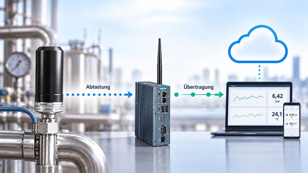
A pressure sensor provides a new measured value every second. However, the process changes only very slowly. Over several minutes, for example, the value fluctuates only between 6.41 and 6.44 bar. Does every individual one-second value really need to be transmitted via the edge gateway to the broker, historian and cloud?
Not necessarily. In many IIoT applications, it makes sense to separate measurement acquisition from data transmission. The sensor or edge system can continue to acquire data at a sufficiently high rate, while downstream systems receive a new value only when the measured variable changes significantly.
This principle is commonly referred to as Change-of-Value, abbreviated COV, or Publish-on-Change. A key parameter is the deadband: it defines how much a measured value must change before a new data record is transmitted or stored.
A well-chosen deadband reduces data volume and communication load without losing relevant process information. A deadband that is too small mainly transmits sensor noise. A deadband that is too large can hide slow trends, reduce dashboard currency and delay the visibility of relevant changes.
What does Change-of-Value mean?
With a fixed transmission interval, a measured value is transmitted regardless of whether it has changed.
For example:
send a new measured value every second
A nearly constant process can therefore generate data records such as:
6.42 → 6.42 → 6.43 → 6.42 → 6.42 → 6.43 bar
For many long-term monitoring applications, these messages contain very little additional information.
With Change-of-Value, the system instead checks how much the current measured value has changed compared with a defined reference value.
A new value is published only when the change reaches or exceeds a specified amount.
In simplified form:
|current value - reference value| ≥ deadband → send
This allows the measuring point to continue being sampled internally at regular intervals without forwarding every individual sample to higher-level systems.
Why are sampling rate and transmission rate not the same?
This distinction is particularly important for a good IIoT architecture.
A system can, for example:
acquire 10 measured values per second
but only:
transmit when a relevant change occurs
or additionally:
send a heartbeat every 5 minutes
The high internal sampling rate may still be required for:
- local alarm evaluation,
- minimum/maximum acquisition,
- rate-of-change calculation,
- diagnostics,
- control,
- detection of short process events.
The transmission rate, on the other hand, answers a different question:
How often does a higher-level system really need to receive a new data record?
A low publication rate therefore does not automatically mean that the sensor itself measures slowly.
What does deadband mean?
The deadband defines the minimum change in a measured value that is considered relevant.
Example:
Last transmitted pressure:
6.40 bar
Deadband:
0.10 bar
New measured values:
| Current value | Change | Transmit? |
|---|---|---|
6.43 bar |
+0.03 bar |
No |
6.47 bar |
+0.07 bar |
No |
6.50 bar |
+0.10 bar |
Yes |
After transmission of 6.50 bar, this value typically becomes the new comparison basis.
However, exactly how a specific protocol, gateway or software module calculates the deadband must be checked for the particular project.
Which value is used as the comparison basis?
This point is particularly important for slowly changing measured variables.
A sensible Change-of-Value method often compares the new measured value with the:
last reported or transmitted value
Example:
Deadband:
0.10 bar
Last transmitted:
5.00 bar
The pressure then slowly increases:
5.02 → 5.04 → 5.06 → 5.08 → 5.10 bar
Each individual change is only 0.02 bar.
Compared with the last transmitted value, however, the total change at the end is:
0.10 bar
and a new value should be transmitted.
If an unsuitable implementation instead compares each value only with the immediately preceding sample, a slow continuous drift could, under certain conditions, remain below the individual change threshold for a very long time.
During system design, it should therefore be clearly established how the specific COV method defines its comparison basis.
Absolute or relative deadband?
A deadband can be defined in different ways.
An absolute deadband uses a fixed engineering unit:
±0.1 bar
or:
±0.2 °C
or:
±5 mm
A relative deadband, on the other hand, can be specified as a percentage of a defined range.
For example:
1 % of 0 ... 10 bar = 0.1 bar
For industrial measured variables, an absolute deadband in engineering units is often particularly transparent because it directly shows what real change is required to trigger a new transmission.
For percentage values, however, it must be clearly documented what the percentage refers to:
- measuring span,
- current measured value,
- last transmitted value or
- another defined reference quantity.
The actual implementation depends on the device or software.
Why must sensor noise be taken into account?
No real sensor produces a mathematically constant numerical value when the process variable is perfectly stable.
A pressure signal can, for example, fluctuate:
6.421 → 6.426 → 6.419 → 6.424 bar
without any relevant change in the actual process.
Possible causes include:
- sensor noise,
- measurement-chain resolution,
- EMC influences,
- small real process fluctuations,
- digitization noise.
If the deadband is set smaller than this normal fluctuation range, Change-of-Value will again result in an almost continuous stream of messages.
The deadband should therefore be sufficiently larger than the normal irrelevant signal variation.
What role does measurement resolution play?
The resolution of the measuring system must also be taken into account.
A sensor may, for example, provide values only in increments of:
0.1 °C
A deadband of:
0.01 °C
would therefore be practically meaningless.
Conversely, the deadband should not be set to a multiple of the relevant process resolution without good reason.
Parameterization should therefore take at least the following into account:
- sensor resolution,
- measurement accuracy,
- normal process fluctuation,
- smallest relevant process change.
What happens if the deadband is too small?
A deadband that is too small hardly reduces the data volume.
Example:
Measured value:
50.00 %
Normal fluctuation:
±0.04 %
Deadband:
0.01 %
Normal measurement noise alone can continuously generate new messages.
Possible consequences include:
- high MQTT message rate,
- unnecessary database entries,
- larger cloud data volumes,
- higher network load,
- unstable-looking dashboards,
- higher energy consumption for wireless or battery-powered devices.
The Change-of-Value function then loses much of its benefit.
What happens if the deadband is too large?
A deadband that is too large can reduce the data volume very effectively, but it can also hide important information.
Example:
Tank level:
50.0 %
Deadband:
5 %
The actual level slowly falls:
50 → 49 → 48 → 47 → 46 %
The higher-level system could continue to display:
50 %
for a long period of time.
The data are not necessarily technically incorrect, but they are not sufficiently current for the intended use.
A deadband that is too large can therefore:
- hide slow trends,
- reduce the quality of maintenance forecasts,
- cause dashboards to become outdated,
- change statistical evaluations,
- delay the visibility of relevant process changes.
Why does Change-of-Value need a heartbeat?
An unchanged measured value should not mean that a higher-level system never receives another message.
Otherwise, after a long period of time it becomes unclear:
Is the value really unchanged?
or:
Has the sensor, gateway or communication failed?
For this reason, combining Change-of-Value with a maximum transmission interval is useful.
Example:
COV deadband = 0.1 bar
Heartbeat = 5 min
This means:
- transmit immediately when a relevant change occurs,
- transmit the current status again after no more than 5 minutes.
This keeps the data point current and monitorable even when the process remains completely constant.
Which timestamp should be transmitted?
With Change-of-Value, a clear time reference is particularly important.
A data record should ideally carry the time at which the relevant measured value was actually acquired or recognized as a change.
The following should not be confused:
- measurement time,
- publication time,
- broker receipt time,
- database write time.
During normal online communication, these times can be very close together.
With buffering or communication interruptions, however, they can differ significantly.
For historian and analysis applications, the original measurement or event time should therefore be preserved wherever possible.
What happens when the quality status changes?
A deadband should normally evaluate only the change in the actual measured value.
If, however, the quality status of a data point changes from:
Good → Bad
this information must be transmitted regardless of whether the numerical value has changed.
Example:
Last value:
6.42 bar · Good
Sensor loses communication:
6.42 bar · Bad
The numerical value is identical.
However, the meaning of the data record has changed completely.
Changes in:
- Good,
- Uncertain,
- Bad,
- device status,
- diagnostic flags
should therefore be handled independently of the normal value deadband logic.
Do not confuse deadband with alarm hysteresis
Deadband for measured-value transmission and hysteresis for an alarm limit serve different purposes.
| Function | Purpose |
|---|---|
| Telemetry deadband | reduces normal measured-value transmissions |
| Alarm hysteresis | prevents repeated switching of an alarm on and off around the threshold |
| Alarm delay | evaluates how long a limit violation must persist |
Ideally, an alarm condition should be evaluated using sufficiently frequently acquired local or unprocessed process values.
It should not depend on whether a telemetry deadband has already happened to trigger a new transmission.
Alarm handling and data reduction should therefore remain separate functions.
Can short peaks be lost with COV?
Change-of-Value alone does not automatically prevent information loss.
An edge system can, for example, measure once per second but publish only relevant changes.
A short pressure peak could occur internally and disappear again before the next regular heartbeat is sent.
Depending on the application, it may therefore additionally be useful to:
- store minimum values,
- store maximum values,
- transmit average values,
- handle peaks as separate events,
- buffer raw data locally for a limited period.
A possible data record could contain, for example:
average = 6.42 bar
min = 6.39 bar
max = 6.91 bar
This ensures that a short peak remains visible even though not every raw sample is stored permanently in the cloud.
Practical example: slowly changing process pressure
A pressure sensor monitors a supply line.
Measuring range:
0 ... 10 bar
Normal operating value:
approx. 6.5 bar
Internal acquisition:
1 value/s
During stable operation, the sensor signal typically fluctuates by:
±0.02 bar
Initially, every value is transmitted via MQTT to the historian.
This generates per measuring point and day:
86,400 messages
even though the process often changes very little for hours.
The edge configuration is therefore changed, for example, to:
Deadband = 0.10 bar
Heartbeat = 5 min
The pressure starts at:
6.40 bar
and changes slowly:
6.42 → 6.44 → 6.46 → 6.48 → 6.50 bar
Only at:
6.50 bar
is a new COV value transmitted.
If the pressure then remains unchanged, the current status is published again no later than the next heartbeat.
Local alarm processing continues independently using the continuously acquired measured values.
This significantly reduces the IT-side data volume while preserving process monitoring, alarm handling and currency checking.
How much can COV reduce the data volume?
The possible reduction depends entirely on the process dynamics.
With a fixed interval of one second:
86,400 values per day and measuring point
are generated.
With a heartbeat every five minutes, the heartbeat alone produces:
288 values per day
plus all actual Change-of-Value events.
For a very stable measured variable, the reduction can therefore be considerable.
For a highly dynamic process, on the other hand, almost every sample may exceed the deadband threshold.
Change-of-Value is therefore particularly useful for slowly changing variables such as:
- tank level,
- room temperature,
- certain process pressures,
- slow temperature processes,
- inventory quantities.
What happens during a communication failure?
An IIoT system should define what happens if the connection to the broker or cloud fails.
One possible strategy is:
- The sensor or edge system continues acquiring data locally.
- Relevant COV events retain their original timestamp.
- Data records are buffered locally.
- They are transmitted after the connection is restored.
It must be ensured that a value transmitted later is not incorrectly treated as if it had only occurred at the time of transmission.
In addition, after a restart or reconnect, the current status should be published explicitly.
This gives the higher-level system a defined starting value again for further Change-of-Value evaluation.
Selecting the deadband systematically
- Define the measured variable and measuring range.
- Determine sensor resolution.
- Determine typical measurement noise or normal process fluctuation.
- Define the smallest technically relevant process change.
- Set the deadband above irrelevant fluctuations.
- Check that the deadband remains small enough for trend and diagnostic requirements.
- Check the comparison basis of the specific COV algorithm.
- Define heartbeat or maximum transmission interval.
- Exclude quality and status changes from the value deadband.
- Handle alarms independently of telemetry reduction.
- Add minimum/maximum or peak acquisition if required.
- Preserve original timestamps.
- Define offline buffering and reconnect behaviour.
- Verify data volume and information quality during pilot operation.
Common mistakes
- Equating sampling rate with transmission interval: A sensor can measure quickly and still transmit only selected values.
- Setting the deadband smaller than normal sensor noise: This results in almost continuous telemetry again.
- Selecting the deadband based only on data costs: The smallest technically relevant process change is decisive.
- Using no heartbeat: An unchanged value then becomes difficult to distinguish from a communication failure.
- Comparing each value only with the previous sample: Depending on the implementation, slow drift may then be handled unfavourably.
- Confusing alarm hysteresis with telemetry deadband: The two functions have different purposes.
- Applying the normal deadband to the quality status: Good → Bad must be transmitted even when the numerical value remains unchanged.
- Generating timestamps only in the cloud system: During buffering, the original measurement time is lost.
- Using Change-of-Value without peak detection: Short relevant extreme values can be missing from condensed long-term data.
- Using a relative deadband without documenting its reference basis: A percentage value is ambiguous without a clearly defined reference.
- Not sending the current status after reconnect: The higher-level system may continue working with an outdated last value.
- Using one deadband for all measured variables: Temperature, pressure, level and vibration have completely different dynamics.
IIoT solutions from field device to cloud
ICS Schneider integrates industrial measuring points from the field device via edge gateways into SCADA, historian and cloud systems.
Typical field interfaces include:
- RS-485 / Modbus RTU,
- HART,
- IO-Link,
- OPC UA,
- Ethernet.
MQTT or HTTPS can be used, among other technologies, for transmission to higher IT levels.
A typical architecture is:
Sensor → field communication → edge gateway → MQTT/HTTPS → historian / dashboard / cloud
The edge system can perform tasks such as:
- scaling,
- timestamping,
- data modelling,
- local alarm processing,
- buffering,
- data aggregation,
- deadband or Publish-on-Change.
Which functions are actually available depends on the gateway, operating system and software configuration being used.
One example of an IIoT device architecture available from ICS is the Siemens SITRANS MS200, which is intended for vibration and temperature monitoring in combination with the SITRANS CC220 gateway.
With such an architecture, it should be clearly defined whether Change-of-Value or deadband is implemented:
- already in the sensor,
- in the gateway,
- in an edge application or
- only in the higher-level system.
Further information can be found under IIoT solutions at ICS Schneider.
Conclusion
A fixed transmission interval is easy to configure, but for slowly changing measured variables it often produces a large number of almost identical data records.
Change-of-Value separates internal measurement acquisition from the actual transmission. A new data record is published only when the measured variable changes by a defined amount.
The correct deadband size is decisive. It should be large enough to prevent sensor noise and irrelevant fluctuations from being transmitted continuously, but small enough to keep technically relevant changes and slow trends visible.
A COV system should also not consist solely of a deadband. A periodic heartbeat ensures that an unchanged process value remains recognizable as current.
Quality changes, diagnostic states and alarms should be handled independently of the normal value deadband. Original timestamps, offline buffering and behaviour after reconnect must also be part of the data strategy.
For robust IIoT telemetry, the following therefore applies: sample sufficiently fast, transmit only relevant value changes, choose a deadband adapted to measurement noise and process dynamics, send a periodic heartbeat and never make status, alarm or quality changes dependent solely on the normal Change-of-Value threshold.
FAQ: Change-of-Value and deadband for IIoT measured values
What does Change-of-Value mean?
With Change-of-Value, a new measured value is transmitted only when the measured variable has changed sufficiently compared with a defined reference.
What is a deadband?
The deadband defines the minimum change in a measured value that triggers a new data record or transmission.
Is deadband the same as hysteresis?
Not necessarily. A telemetry deadband controls when measured values are transmitted. Alarm hysteresis, on the other hand, controls when an alarm is activated or reset.
Does a sensor need to measure more slowly with COV?
No. The sensor or edge system can continue acquiring data at a high rate. Only the publication rate is reduced.
How large should the deadband be?
It should be above the normal irrelevant signal variation while remaining smaller than the smallest technically relevant process change.
What happens if the deadband is too small?
Sensor noise and small process fluctuations continuously generate new messages. As a result, the desired data reduction is limited.
What happens if the deadband is too large?
Slow changes may not be transmitted until later. Trends and current process states can therefore become less visible.
Why does Change-of-Value need a heartbeat?
A heartbeat ensures that an up-to-date status is transmitted regularly even when the measured value remains unchanged. This makes it easier to distinguish a stable process from a communication failure.
Should a quality change trigger a COV event?
Yes. If the status changes, for example, from Good to Bad, this change should be transmitted independently of the numerical deadband.
Can short peaks be lost with COV?
Yes, if no additional peak, minimum/maximum or event logic is present. Relevant extreme values should therefore be captured separately depending on the application.
Is an absolute or percentage deadband better?
That depends on the application. An absolute deadband in engineering units is often particularly transparent. With a percentage deadband, the reference basis must be clearly defined.
Where should the COV logic be executed?
Depending on the architecture, it can be implemented in the sensor, PLC, edge gateway or higher-level application. For fast local alarms, safety- or process-relevant evaluation should not depend on a remote cloud connection wherever possible.
Which IIoT solutions does ICS Schneider offer for this?
ICS Schneider integrates sensors and field devices via interfaces such as Modbus RTU, HART, IO-Link, OPC UA or Ethernet into edge, SCADA and cloud architectures and supports data modelling, topic design, timestamping, alarms, buffering and data preprocessing.