


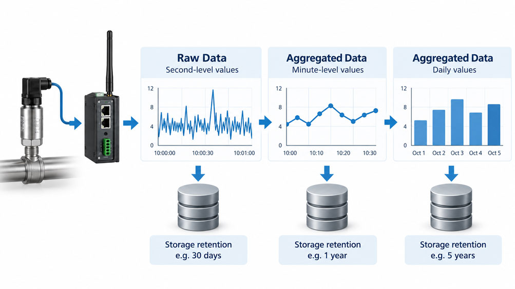
An industrial company monitors the pressure and temperature of several machines. Sensor readings are collected every second through a PLC and an edge gateway and transmitted to a central IIoT platform. During the first few weeks, the system operates without problems. Measurements are displayed in real time on dashboards, short pressure fluctuations can be tracked, and maintenance personnel can investigate historical operating conditions.
After several months, however, the database has grown considerably. More and more measuring points are integrated, additional machines transmit their data, and historical analyses require increasing resources. Preparing an energy report covering the previous year suddenly requires processing millions of individual data points, even though hourly or daily statistics would often be sufficient for this type of analysis.
The obvious solution is to aggregate older data. For example, numerous individual second-level readings can be combined into minute averages together with their corresponding minimum and maximum values. Additional daily statistics can be calculated from these values for long-term analysis. High-resolution raw data is then retained for only a limited period.
However, this type of data aggregation must be planned carefully. If only average values are stored, short pressure peaks, temperature limit violations or other relevant process events may disappear. Data gaps may also be concealed within apparently plausible daily averages. This is particularly critical if the aggregated data is later required for root cause analysis, quality documentation or the investigation of equipment faults.
Another question is when raw data may actually be deleted. An automatic retention policy can permanently remove data even though aggregation has not yet been completed or late-arriving measurements still need to be included. Data acquisition, aggregation, retention and deletion must therefore be considered as interconnected processes.
This technical article explains how raw data, minute-level values and daily statistics can be stored with different retention periods. It focuses on data models, timestamps, aggregation functions, data quality, time windows, edge buffering and the safe deletion of older measurements. A calculation example involving 100 industrial measurement channels demonstrates how significantly the number of stored records can be reduced through tiered retention. Typical faults, suitable IIoT architectures and appropriate measurement and communication solutions from the ICS product range are also discussed.
Table of Contents
- Define the Measurement Task and Future Information Requirements
- Distinguish Raw Data, Validated Measurements and Aggregated Data
- Understand Retention as a Separate Data Storage Policy
- Store Second-, Minute- and Daily-Level Values for Different Purposes
- Distinguish Measurement, Transmission and Storage Intervals
- Correctly Calculate Average, Minimum, Maximum and Sample Count
- Clearly Define Time Windows, Timestamps and Time Zones
- Calculation Example: Data Volume for 100 Measurement Channels Over Five Years
- Preserve Short Pressure Peaks and Other Extreme Values During Aggregation
- Document Data Gaps, Invalid Measurements and Completeness
- Distinguish Arithmetic and Time-Weighted Averages
- Perform Multi-Level Aggregation Without Systematic Calculation Errors
- Define a Data Model for Raw Measurements and Aggregates
- Separate Measurement Time, Reception Time and Aggregation Period
- Consider Edge Gateways, Local Buffering and Delayed Data Transmission
- Select Time-Series Databases, Historians and Separate Retention Policies
- Safely Coordinate Aggregation Tasks and Automatic Data Deletion
- Archive Alarms, State Changes and Fault Events Separately
- Version Units, Scaling and Calculation Methods
- Systematically Implement and Verify Tiered Data Retention
- Identify Typical Errors in Data Aggregation and Retention
- Suitable IIoT Measurement Technology and Integration Solutions from ICS Schneider
- Conclusion: Plan Retention According to Information Value Rather Than Data Volume Alone
- Frequently Asked Questions About Raw Data, Aggregation and Retention
1. Define the Measurement Task and Future Information Requirements
Before defining a retention strategy, it is necessary to understand how the stored measurement data will be used in the future.
A pressure sensor may, for example, be used exclusively to display the current operating pressure. However, the same measured quantity may also be required to analyse pressure peaks, calculate operational performance indicators or document specific process conditions.
These tasks have different requirements regarding temporal resolution and retention periods.
For a current process display, one measurement per second may be useful.
For a long-term trend report, minute-level or hourly values may be sufficient.
For the retrospective investigation of a short machine fault, however, the original high-resolution measurements may be required.
Retention should therefore not be defined identically for all measurement channels without considering their individual requirements.
Instead, the requirements of each relevant group of measured quantities should be evaluated.
It is particularly important to distinguish between normal process values and information relevant to safety or quality.
A long-term temperature trend may be adequately described by daily averages.
However, investigating a brief temperature limit violation may require minimum and maximum values, event timestamps or high-resolution measurements.
Possible legal or contractual documentation requirements must also be considered.
A technically appropriate example of data retention does not automatically satisfy the applicable archival obligations of a particular industry.
The measurement task therefore determines which information must be preserved and which temporal resolution may eventually be discarded.
2. Distinguish Raw Data, Validated Measurements and Aggregated Data
IIoT applications frequently produce several successive forms of data.
The first level consists of the originally acquired measurements.
In data storage applications, these are generally referred to as raw data.
Depending on the system, they may consist of digital sensor readings, transmitted process values or measurements that have already been scaled by the field device.
The term raw data therefore does not automatically mean that unprocessed electrical ADC counts are available.
What matters is which data is stored as the unchanged input values of the archival system being considered.
A second level may consist of quality-checked or normalised measurement data.
At this stage, units may be standardised, invalid measurements flagged or values assigned to a consistent data model.
These processing steps should remain traceable.
The third level comprises aggregated data.
During aggregation, several individual measurements within a time window are summarised using suitable statistical values.
For example, 60 one-second readings can be used to calculate a minute average, minimum and maximum.
Daily values can subsequently be derived from these minute statistics, provided that the aggregation method is suitable.
This process is also referred to as aggregation or downsampling.
It often significantly reduces the amount of data.
However, information not included in the stored aggregates is lost.
For example, a minute average cannot reliably reveal the exact moment within that minute when a pressure peak occurred.
A carefully designed retention strategy therefore explicitly defines which information must be preserved at each aggregation level.
3. Understand Retention as a Separate Data Storage Policy
Retention refers to the defined period for which data is kept.
In a time-series database, for example, measurements can be deleted automatically once they exceed a specified age.
The corresponding rule is called a retention policy.
A simple example is to store high-resolution raw data for 30 days.
Older raw data is removed from the corresponding storage area once this period has expired.
Previously calculated minute and daily statistics can be retained independently for much longer periods.
This strategy reduces long-term storage requirements without losing all information about historical process behaviour.
It is particularly important to distinguish between data aggregation and retention.
Aggregation generates new statistical records from existing measurements.
Retention, on the other hand, determines when records are removed from a particular storage level.
Both processes must be coordinated.
If raw data is deleted before the associated aggregates have been fully generated and verified, historical information may be lost permanently.
Automatic retention is also not a substitute for data backup.
Backups are intended to restore data after faults or data loss. Retention determines the normal lifecycle of data within the archive.
Both functions require their own policies.
Retention periods should therefore be treated as explicitly documented operating settings rather than arbitrary database defaults.
4. Store Second-, Minute- and Daily-Level Values for Different Purposes
A tiered measurement data archive uses several temporal resolutions in parallel.
One possible structure consists of high-resolution raw data, minute-level aggregates and daily statistics.
Each data level serves a different purpose.
| Data Level | Temporal Resolution | Example Retention Period | Stored Information | Typical Purpose |
|---|---|---|---|---|
| Raw data | 1 second | 30 days | Individual measurement, measurement timestamp, quality status, measurement point ID | Troubleshooting, high-resolution trends, short-term process diagnostics |
| Minute-level values | 1 minute | 365 days | Average, minimum, maximum, valid sample count, data quality | Shift analysis, maintenance, medium- and long-term trend analysis |
| Daily values | 1 calendar day | 5 years | Suitable daily statistics, extreme values, completeness and, where appropriate, totals | Long-term reporting, energy analysis, equipment comparisons and historical KPIs |
The retention periods shown are freely chosen technical examples.
They do not represent legal requirements or universally applicable recommendations for every measuring point.
Certain applications may require high-resolution data to be stored for considerably longer periods.
Conversely, slowly changing process quantities may not require measurements every second.
The temporal levels must therefore be derived from the actual measurement task.
Aggregation functions may also differ depending on the measured quantity.
For a continuous pressure signal, average, minimum and maximum can be useful.
For an energy meter, however, the difference between two meter readings or a correctly calculated consumption total may be decisive.
For digital switching states, the active duration, number of state changes and alarm events may be more important than a conventional arithmetic average.
A suitable retention strategy therefore considers not only temporal resolution but also the meaning of each type of measurement.
5. Distinguish Measurement, Transmission and Storage Intervals
In an IIoT architecture, the terms measurement interval, transmission interval and storage interval are frequently treated as equivalent.
Technically, however, they may represent different time intervals.
The measurement interval describes how frequently a sensor or controller acquires a new reading.
The transmission interval determines how frequently values are forwarded to a higher-level system.
The storage interval describes the temporal resolution at which measurements or aggregates are stored in the archive.
For example, a sensor may measure internally every second while a wireless module transmits one value every 60 seconds.
If only the latest individual reading is transmitted, the higher-level system does not automatically receive all 60 preceding second-level measurements.
Storing the transmitted reading as a minute value cannot reconstruct the missing individual measurements.
The situation is different if the field device calculates suitable statistics itself or transmits all individual readings together with their original timestamps.
The information actually available then depends on the device and the communication protocol.
Distinguishing between measurement and wireless transmission can be particularly important for wireless IIoT sensors.
Transmission intervals are often selected to reduce energy consumption and the volume of wireless data.
A shorter internal measurement interval therefore does not automatically mean that the same volume of historical data is available in the cloud.
Retention planning must explicitly establish which measurements the archive actually receives.
The intended aggregation resolution must not be confused with a higher physical measurement resolution than the system actually provides.
6. Correctly Calculate Average, Minimum, Maximum and Sample Count
The choice of aggregation function is crucial to the usefulness of aggregated measurement data.
One frequently used statistical value is the arithmetic mean.
For n valid measurements xi, it is calculated as follows:
x̄ = (Σ xi) / n
The average describes the mean level of the measurements included in the calculation.
However, it does not contain complete information about their distribution within the time window.
For example, a single high pressure reading may be largely concealed by numerous lower readings in the average.
Suitable process quantities should therefore also retain minimum and maximum values.
The minimum represents the smallest valid measurement considered within the respective window.
The maximum represents the largest valid measurement recorded within that window.
The number of measurements actually used is also important.
It helps assess the reliability of a calculated average.
With measurements taken every second, 60 readings are normally expected within a fully recorded minute.
If only 45 of these values are valid, this deviation should not be concealed.
Another important attribute is the quality status.
It describes, for example, whether all measurements were valid or whether certain readings were excluded because of sensor faults or communication errors.
Data quality must also be considered when determining extreme values.
A sensor reading flagged as invalid must not automatically be treated as the actual process maximum without an appropriate rule.
The OPC UA specification explicitly defines different functions for historical aggregates, including average, time-weighted average, minimum, maximum and other statistics, together with rules for evaluating data quality.
Technically reliable minute-level values therefore often require several related statistical attributes.
7. Clearly Define Time Windows, Timestamps and Time Zones
During aggregation, measurements are assigned to a specific time interval.
Such an interval is frequently referred to as a time window or time bucket.
Processing requires an unambiguous definition of where each window begins and ends.
One common definition uses an interval that includes its starting point but excludes its ending point.
For example:
[10:00:00, 10:01:00)
This time window includes measurements from 10:00:00 onwards but excludes measurements timestamped exactly 10:01:00.
This assignment prevents values located at window boundaries from being counted twice.
It must also be defined which timestamp is stored for the aggregate.
The beginning of the time window is frequently used.
A minute-level value timestamped 10:00:00 can therefore describe the interval from 10:00:00 up to, but not including, 10:01:00.
The timestamp does not necessarily represent the actual measurement time of an individual reading.
Daily values require even more careful consideration.
A technical day consisting of exactly 24 hours is not always equivalent to a local calendar day.
Because of daylight saving time changes, a local calendar day may contain 23 or 25 hours.
A consistent UTC time base can be useful for data storage.
However, if daily statistics must refer specifically to local calendar days, the relevant time zone and calendar boundaries must be handled correctly.
The origin of the timestamp is also important.
A timestamp may refer to the time of physical measurement, reception by the gateway or arrival in the cloud.
These timestamps are not automatically equivalent.
Their precise meaning should therefore form part of the data model.
8. Calculation Example: Data Volume for 100 Measurement Channels Over Five Years
An industrial test bench has 100 measurement channels.
Each channel provides exactly one measurement per second throughout the period being considered.
For this simplified calculation, continuous operation around the clock is assumed.
Years containing 365 days are also assumed.
Leap years, data gaps and additional event records are excluded from this example.
Without data aggregation, the following number of measurements would be generated per day:
Nday = 100 · 86,400 = 8,640,000 measurements
Over five years:
N5 years = 100 · 86,400 · 365 · 5
N5 years = 15,768,000,000 measurements
This corresponds to more than 15.7 billion individual measurement records.
Now consider a tiered retention strategy.
Raw data is retained for 30 days.
Minute-level aggregates are also stored for 365 days.
Daily aggregates remain available for five years.
For the following calculations, it is assumed that exactly one aggregate record is generated for each measurement channel and complete time window.
This record may contain several statistical values, such as average, minimum, maximum and valid sample count.
For raw data:
Nraw data = 100 · 86,400 · 30 = 259,200,000
For minute-level values:
Nminutes = 100 · 1,440 · 365 = 52,560,000
For daily values:
Ndays = 100 · 365 · 5 = 182,500
| Storage Strategy | Resolution | Retention | Stored Records |
|---|---|---|---|
| Raw data archive | 1 second | 30 days | 259,200,000 |
| Minute-level archive | 1 minute | 365 days | 52,560,000 |
| Daily archive | 1 day | 5 years | 182,500 |
| Total tiered storage | Multiple resolutions | Different for each data level | 311,942,500 |
| Alternative: retain all raw data for five years | 1 second | 5 years | 15,768,000,000 |
In this simplified model, the tiered strategy requires approximately 312 million records.
Storing all second-level readings for five years would instead require approximately 15.8 billion records.
The number of stored records is therefore reduced by approximately 98 %.
However, it is important to recognise that this comparison only considers the number of records.
A minute-level aggregate containing several statistical values may require more storage space than a single raw measurement.
Timestamps, database indexes, compression, metadata and the actual storage architecture also affect storage requirements.
The calculated reduction in record count therefore does not automatically correspond to the same percentage reduction in database size or operating costs.
The calculation also assumes that minute and daily aggregates are successfully generated and stored before the required raw data expires.
The technical suitability of this aggregation strategy remains particularly important.
For process events requiring second-level data even after several years, longer raw data retention or a separate event archive may be necessary.
The calculation example describes one possible technical architecture and does not represent universally applicable retention periods.
9. Preserve Short Pressure Peaks and Other Extreme Values During Aggregation
One particular risk of data aggregation is that short events may disappear within an average.
For example, a hydraulic system may operate at 120 bar for almost an entire minute.
However, a measured pressure value of 180 bar occurs for a brief moment.
If only the minute average is stored, this short-term load may no longer be identifiable later.
Yet this extreme value may be crucial for certain condition monitoring and wear analyses.
Minimum and maximum values should therefore also be preserved for suitable measured quantities.
A minute-level aggregate could, for example, contain the following information:
Average: 121.0 bar
Minimum: 119.5 bar
Maximum: 180.0 bar
Valid sample count: 60
The figures describe an illustrative operating condition.
It may also be useful to store the actual timestamp of the extreme value.
A maximum assigned only to the beginning of a minute window does not reveal exactly when the pressure peak occurred within that minute.
The timestamps of the relevant minima and maxima may therefore be important for subsequent root cause analysis.
However, the physical sampling rate must also be considered.
If a sensor measures only once per second, much shorter pressure peaks occurring between sampling points may remain undetected.
A stored maximum therefore initially represents the highest valid value actually recorded.
It is not necessarily equal to the absolute physical maximum of the entire process.
Very fast pressure events may require correspondingly faster sensors and data acquisition systems.
Subsequent data aggregation cannot compensate for an inadequate original sampling rate.
10. Document Data Gaps, Invalid Measurements and Completeness
A stored average is only meaningful when the quality of the underlying measurement data is known.
Missing, invalid or late-arriving measurements are particularly important.
A simple example considers a measuring point with a specified sampling interval of one second.
Within one minute, 60 measurements would therefore be expected.
If only 50 valid measurements are available because of a communication fault, the numerical completeness is:
Completeness = 50 / 60 · 100 % ≈ 83.3 %
An average calculated from the 50 available readings may be mathematically correct.
However, it does not necessarily represent the entire period.
It would be particularly problematic to treat the missing period as normal process operation without any indication.
Missing values must also not automatically be replaced with zero.
For pressure measurement, this could produce an artificially low average.
Suitable methods therefore distinguish between valid readings, invalid readings and completely missing data.
An aggregate should, where appropriate, contain the number of valid values, the expected number of values and a corresponding quality status.
The actual calculation of completeness depends on the type of data source.
With event-driven transmission, there is not necessarily a fixed sampling interval with an expected number of readings.
For irregular sampling, evaluating time coverage may be more appropriate than simply counting the available data points.
The corresponding rules must be clearly defined for automatic evaluation.
It is particularly important that invalid aggregates are not silently processed as fully valid daily statistics.
An incomplete minute must be appropriately accounted for or flagged during daily aggregation.
11. Distinguish Arithmetic and Time-Weighted Averages
Different definitions of average are available for aggregating industrial measurements.
With evenly spaced, valid individual readings, an arithmetic average may adequately describe the measurements within the period being considered.
However, this interpretation is not always correct when sampling intervals are irregular.
For example, a pressure sensor may transmit values infrequently under stable process conditions but transmit more frequently during rapid changes.
A simple average of all received readings then assigns greater weight to periods containing more data points.
This does not necessarily correspond to the actual time distribution of the pressure.
A time-weighted average may be more suitable for such applications.
This takes into account how long certain readings or interpolated signal values apply within the time window.
The actual calculation depends on the signal model used.
With a stepwise signal interpretation, for example, a measurement is assumed to remain valid until the next update.
For a continuous signal, linear interpolation between measurement points may be appropriate under suitable conditions.
Both methods can produce different results.
The selected calculation method must therefore match the measured quantity and the sampling method.
The treatment of missing time periods must also be clearly defined.
A long data gap must not be transformed into an apparently complete process history through arbitrary interpolation without appropriate justification.
The OPC UA specification therefore explicitly distinguishes between the ordinary Average aggregate and various time-weighted average methods.
For long-term retention, the aggregation method actually used should be recorded.
A numerical daily average without information about its calculation method may have limited value for later interpretation.
12. Perform Multi-Level Aggregation Without Systematic Calculation Errors
A tiered IIoT architecture can generate daily values from existing minute-level values.
This approach reduces the number of raw measurements that must be processed directly.
However, not all statistical values can be aggregated repeatedly without special consideration.
Correct calculation of averages is particularly important.
If every minute contains the same number of valid, evenly spaced measurements, the arithmetic mean of the minute averages can equal the average of all individual measurements.
However, if some minutes contain missing readings, a simple average of the minute averages may be incorrect.
To correctly combine arithmetic averages, the number of readings used and their corresponding sums should therefore be considered.
The calculation can be expressed approximately as follows:
x̄total = Σ (ni · x̄i) / Σ ni
Here, ni represents the number of valid measurements and x̄i the average of the respective subinterval.
For time-weighted averages, suitable time weights or the corresponding integrals and valid time durations must be used instead.
Under suitable conditions, minima and maxima can be combined more easily across several aggregation levels.
For example, the daily minimum can be calculated as the minimum of the valid minute-level minima.
The daily maximum is correspondingly obtained from the maximum of the valid minute-level maxima.
This approach preserves the extreme values actually recorded, provided that the underlying time windows and quality rules are correct.
The situation is different for statistical distributions.
In general, a median or specific percentile cannot be reconstructed exactly from the averages of individual minutes.
If such analyses are required in the long term, suitable additional statistics, distribution information or specialised statistical data structures must be retained.
Aggregation must therefore be checked for future analytical requirements before the raw data is deleted.
13. Define a Data Model for Raw Measurements and Aggregates
Storing only numerical values and timestamps is insufficient for reliable long-term data storage.
Particularly when several measuring points and aggregation levels are involved, the meaning of every record must be unambiguous.
A suitable raw data record may contain a stable measurement point ID, measured value, unit, acquisition timestamp and quality status.
Additional information about the sensor version, data source and scaling used may also be necessary.
An aggregate requires further attributes.
These include the time window used, aggregation type and the quantity of data actually considered.
An example minute-level aggregate could have the following structure:
Measurement point: pressure.line_01
Window start: 2026-10-13T08:00:00Z
Window duration: 60 s
Average: 8.42 bar
Minimum: 8.10 bar
Maximum: 9.35 bar
Valid samples: 60
Expected samples: 60
Quality: valid
Aggregation: avg/min/max, Version 1
This is an illustrative data model rather than a universally prescribed format.
Clearly identifying the temporal resolution is particularly important.
A second-level reading and a daily average must not be treated as identical types of data points without appropriate metadata.
Separate tables, buckets or database storage areas may also be useful.
The actual structure depends on the chosen storage platform.
However, stable measurement point IDs and documented aggregation semantics should remain traceable regardless of the database software used.
14. Separate Measurement Time, Reception Time and Aggregation Period
In a distributed IIoT architecture, significant delays may occur between physical measurement and central storage.
For example, a sensor may acquire a measurement at 10:00:05.
The edge gateway may not receive it until 10:00:06.
If a wireless or internet connection also fails, the measurement may arrive in the central database much later.
The timestamp used is therefore critical for subsequent time-based analysis.
The original physical acquisition time should be preserved wherever it is reliably available from the data source.
The reception timestamp may additionally be stored for communication diagnostics.
These two timestamps serve different purposes.
Particularly with late-arriving measurements, the cloud reception time must not automatically replace the original measurement time.
Otherwise, the readings may be assigned to the wrong minute or daily window.
Such a shift can alter historical process trends and make it more difficult to correlate alarm events in time.
The system time base must therefore be defined and appropriately synchronised.
Depending on the requirements, NTP, PTP or timestamps from an upstream controller or sensor system may be used.
The required timing accuracy depends on the measurement task.
A slowly changing level measurement may require different timing accuracy from the correlation of rapid machine events.
The origin of the timestamp must therefore remain traceable in aggregated data as well.
A more detailed explanation is available in the ICS technical article Timestamps for IIoT Measurement Data: Sensor, PLC or Gateway?.
15. Consider Edge Gateways, Local Buffering and Delayed Data Transmission
An edge gateway connects industrial sensors and controllers to higher-level IT or cloud systems.
Depending on the architecture, it can acquire and scale measurements, assign timestamps and process data before transmission.
Local aggregation may also be useful.
For example, a gateway can calculate suitable minute-level statistics from regularly acquired second-level readings.
This can reduce the amount of data transmitted across the network.
However, it must be established whether the original second-level measurements will still be required later.
If the gateway transmits only a minute average and immediately discards the second-level values, subsequent detailed analyses can no longer access the original data.
Additional local raw data buffering may therefore be useful for critical process variables.
Behaviour during communication interruptions is particularly important.
A robust IIoT architecture should define which data the gateway stores temporarily when the connection is unavailable.
Buffer capacity must match the maximum intended offline duration and the expected data volume.
After connectivity is restored, buffered records can be transmitted according to the specified procedure.
The original timestamps and data quality information must be preserved.
Records should also have unique identifiers to prevent unwanted duplicates during repeated transmission.
The handling of late-arriving data must also be defined.
If a minute aggregate has already been calculated before all original measurements have arrived, it may need to be updated later.
Retention must allow a sufficiently large processing window for this purpose.
Local buffering and long-term data retention are therefore different but closely related functions.
16. Select Time-Series Databases, Historians and Separate Retention Policies
Different systems are used to store industrial measurement data.
These include conventional process data historians, relational databases with time-series functions and specialised time-series databases.
The selected platform influences how aggregation and retention are implemented technically.
A suitable system should support different temporal resolutions with independent retention policies.
Separating raw data from aggregated data can be particularly advantageous.
For example, high-resolution measurements can be stored in an area with a short retention period.
Minute and daily aggregates can be stored in separate areas with longer retention periods.
For certain product versions, InfluxDB describes downsampling using time-based aggregation tasks and separate storage areas with different retention periods.
TimescaleDB also provides functions for continuous aggregates and automatic data retention.
However, these features are specific to the platform and software version.
The actual configuration must therefore follow the documentation for the database being used.
One particularly important question is how aggregates are updated retrospectively.
If late measurements arrive or historical data is corrected, the corresponding time windows may need to be recalculated.
Some systems handle such changes automatically within defined refresh windows.
Other architectures require separate data processing tasks.
Write load, compression, query performance, fault tolerance and export capabilities are also relevant selection criteria.
The database is therefore only one component of the overall architecture.
A reliable long-term archive requires the coordinated combination of data acquisition, data modelling, aggregation, quality assurance and retention.
17. Safely Coordinate Aggregation Tasks and Automatic Data Deletion
Older raw data should only be deleted automatically once it is no longer required for the intended aggregations.
Correct timing is particularly important for continuous data aggregation.
For example, an aggregation task may regularly calculate completed minute windows.
Another task generates daily statistics from these values.
Only then should the corresponding raw data level expire according to its defined retention period.
This simple sequence becomes more complex when measurements arrive late.
For example, raw data stored during a network outage may not be transmitted to the database until the following day.
If the corresponding aggregates have already been finalised, these measurements may be missing from the historical statistics.
A robust architecture therefore requires a defined strategy for late-arriving data.
This may involve sufficiently large refresh windows, recalculations or the controlled finalisation of previously completed time windows.
Subsequent correction of measurement data may also require aggregation to be performed again.
It is particularly important that raw data retention remains compatible with these refresh windows.
TimescaleDB explicitly documents that continuous aggregates may also lose data under certain conditions if a refresh window is applied to raw data that has already been deleted.
To preserve aggregated historical values permanently, the refresh range must be limited appropriately or coordinated with raw data retention.
InfluxDB also points out that downsampling tasks must be completed before the raw data retention period expires.
Automatic deletion should therefore be supported by appropriate checks.
The mere expiry of a retention period does not prove that all required aggregates have been generated completely.
Regular completeness checks can be useful, particularly for long retention periods.
18. Archive Alarms, State Changes and Fault Events Separately
Continuous process measurements and discrete events serve different purposes.
For example, a pressure sensor may provide a new reading every second.
An alarm, on the other hand, is generated only when a particular condition is detected.
Such events should not be described exclusively by ordinary averages.
A brief alarm condition may disappear completely within a minute average.
During fault investigations, it is often particularly important to know when the condition started, how long it lasted, and when it ended or was acknowledged.
A suitable event archive can therefore contain additional information.
Examples include event ID, measurement point ID, event type, timestamp, limit value, actual measurement, status and, where applicable, acknowledgement information.
Communication failures and changes to device configurations can also be recorded as events.
For subsequent diagnosis, it may be useful to retain relevant high-resolution raw data surrounding certain events for longer periods.
This type of event-dependent archiving is frequently referred to as event retention or event-based storage.
For example, second-level readings from normal operation may be deleted after a defined period, while high-resolution data from specific fault intervals is preserved for longer.
Such functionality must be explicitly implemented.
It does not arise automatically from a conventional time-based retention policy.
Event retention periods must also be determined according to the actual requirements.
For safety-related functions, a distinction must be made between the actual reliable local alarm or protection function and the subsequent archival of the event.
An IIoT cloud must not be used as the sole protective mechanism without appropriate safety-related design.
19. Version Units, Scaling and Calculation Methods
Industrial measurement data may be stored for many years.
During this time, sensors may be replaced, measuring ranges changed or data acquisition systems modernised.
The units and scaling used may also change.
For example, a pressure value may initially be stored in bar and later processed in pascals.
Without appropriate metadata, historical measurements may be interpreted incorrectly.
For aggregated data, the version of the aggregation method is also relevant.
For example, a system may initially calculate arithmetic averages and switch to time-weighted averages after a software update.
The resulting values are not necessarily identical.
If both calculation methods are stored in the same historical data series without appropriate identification, misinterpretation may result.
Important changes to calculation definitions should therefore be documented.
These include the aggregation function, time window definition, data quality rules and, where appropriate, the software version used.
The handling of missing measurements should also remain traceable.
If data gaps were previously filled through interpolation but are later explicitly stored as missing data, this may significantly affect historical statistics.
These differences must be identifiable for reliable long-term use.
Versioning therefore applies not only to individual measurements but also to the rules used to generate aggregated values.
A more detailed explanation of units and scaling is available in the ICS technical article Versioning Units and Scaling in Measurement Data: Permanently Avoiding Bar, Pa and Raw Value Errors.
20. Systematically Implement and Verify Tiered Data Retention
Introducing different retention periods should be carried out as a coordinated technical process.
The following steps describe a general procedure for planning and commissioning an industrial measurement data archive.
- Inventory measuring points: Identify all relevant sensors, measurement channels, controllers and data sources.
- Define measurement tasks: Establish which data is required for current monitoring, troubleshooting, reporting and long-term evaluation.
- Check retention obligations: Consider contractual, organisational and, where applicable, legal requirements for data archiving.
- Document acquisition intervals: Record actual measurement, polling and transmission intervals separately.
- Define the measurement data model: Specify stable measurement point IDs, units, timestamps and quality information.
- Verify the time base: Document the origin and synchronisation of measurement timestamps and the time zone used.
- Define the raw data level: Specify which original data is stored and at what temporal resolution.
- Select aggregation methods: Determine suitable averages, extreme values, totals or other statistics for each measured quantity.
- Define time windows: Clearly specify the beginning, end, duration and timestamp assignment of minute and daily intervals.
- Define quality rules: Document how invalid readings, data gaps and incomplete windows are handled.
- Set retention for each level: Define separate retention periods for raw data, minute-level values and daily statistics.
- Consider event data: Provide separate archival policies where necessary for alarms, state changes and faults.
- Estimate storage requirements: Consider expected data volumes, statistics per aggregate and database overhead.
- Plan edge buffering: Specify the local storage capacity needed for anticipated communication interruptions.
- Handle late-arriving data: Define delayed transmission, duplicate detection and any necessary recalculation of historical time windows.
- Configure aggregation tasks: Set up processing in the designated time-series database or data platform.
- Coordinate retention policies: Ensure that required calculations and updates are completed before raw data deletion.
- Compare results: Verify aggregated values against suitable raw data intervals, particularly checking minimum, maximum and completeness.
- Test fault conditions: Investigate communication outages, late-arriving records, incomplete windows and failed aggregation tasks.
- Document production operation: Record retention periods, data models, aggregation versions, test results, responsibilities and changes in a traceable manner.
It is particularly important that automatic deletion policies are not applied to an existing historical dataset without prior verification.
Before activation, their effects on existing data and any associated reports must be evaluated.
It may be useful to verify aggregation and retention rules using suitable test data before introducing them into production.
Complete quality assurance involves not only calculating individual averages correctly but also ensuring the long-term availability of the required data.
Regular checks of aggregation tasks, storage utilisation and data completeness are therefore part of ongoing operation.
21. Identify Typical Errors in Data Aggregation and Retention
Errors in a retention architecture frequently arise not during the initial acquisition of measurements but during subsequent processing or deletion.
The following overview shows typical observations and suitable diagnostic approaches.
| Observation | Possible Cause | Suitable Check |
|---|---|---|
| Short pressure peaks are no longer visible after aggregation | Only average values were stored | Check minimum and maximum values, event data and necessary raw data retention |
| The daily average differs from the average of all raw data | Minute averages were combined without appropriate weighting | Verify aggregation using valid sample counts or suitable time weights |
| Daily statistics appear complete even though several hours are missing | Data gaps and incomplete time windows were not flagged | Check completeness and quality information in the aggregates |
| Historical minute-level values disappear after raw data retention expires | Aggregation or refresh policies are not correctly coordinated with deletion | Check retention, refresh windows and database behaviour |
| Measurements appear at incorrect times after a network outage | Cloud reception time was used instead of the original measurement timestamp | Investigate timestamp origin and delayed transmission procedures |
| Late-arriving data does not change historical statistics | Previously completed windows are not recalculated | Check late-data handling and refresh policies |
| Some data points appear twice in the archive | Repeated transmission without suitable record identification | Check duplicate detection, measurement point IDs and timestamp processing |
| Long-term trends show unexpected jumps after sensor replacement | Unit, scaling or sensor configuration has changed | Check metadata, conversion and historical configuration versions |
| Minute-level storage remains unusually large despite raw data deletion | Aggregates contain additional statistics, indexes or insufficient compression | Analyse actual storage requirements and database structure |
| Local daily values are missing or duplicated after daylight saving time changes | Time windows were defined without clear time zone rules | Check UTC time base, local calendar windows and daylight saving time handling |
| An alarm event is no longer visible in the long-term trend | Discrete events were processed only as averages | Check separate event archiving and event-based raw data retention |
| Historical reports show different values after a software update | Aggregation functions or quality rules have changed | Evaluate calculation versions and any necessary historical recalculation |
The table describes typical causes and suitable diagnostic approaches.
A definitive fault diagnosis must be based on the actual data architecture.
It is particularly important to distinguish between a measurement that was never acquired, a discarded value and a record that was deleted later.
These three conditions may appear similar in an inadequately documented database, but their causes are different.
For a reliable historical measurement record, data origin, processing and retention must therefore remain traceable together.
22. Suitable IIoT Measurement Technology and Integration Solutions from ICS Schneider
22.1 ICS IIoT Solutions: From Sensors and Edge Gateways to Long-Term Archives
ICS Schneider supports the manufacturer-independent integration of industrial measuring instruments into IIoT, SCADA and cloud systems.
Its range of services includes sensors, data connectivity, edge gateways, data modelling and integration with higher-level IT/OT systems.
Depending on the application, RS-485/Modbus RTU, HART, IO-Link, OPC UA or Ethernet may be used as interfaces at field level.
MQTT and HTTPS are among the available options for communication with higher-level systems.
An edge gateway can acquire and scale measurements, assign timestamps and process them according to the intended system architecture.
Local alarm functions and data buffering may also be implemented.
The actual functions depend on the selected gateway hardware and software architecture.
Multi-level retention with separate second-, minute- and daily-level values must therefore be specified as a function of the complete system architecture and cannot automatically be attributed to every gateway.
ICS Schneider supports the selection of components, data modelling, interface integration and documentation.
Further information is available under IIoT Solutions.
22.2 IDCT531: Digital Pressure Sensor with RS-485 and Modbus RTU
The IDCT531 is an industrial pressure sensor with a digital RS-485 interface and Modbus RTU communication.
The sensor is available with nominal pressure ranges from 0 … 100 mbar to 0 … 400 bar.
The documented accuracy is 0.25 % FSO.
The series offers good temperature performance and high long-term stability.
Its digital interface allows measurements to be polled by a suitable controller or edge gateway.
The actual possible polling frequency depends on the sensor update rate, the communication method and the complete bus configuration.
The IDCT531 is therefore suitable for consideration in industrial pressure monitoring and IIoT applications.
For long-term data archiving, it must also be defined how measurements acquired via Modbus are timestamped and stored.
Retention and aggregation are not automatically provided merely because a Modbus interface is available.
These functions must be implemented by the connected data acquisition or IT system.
22.3 WIKA PEW-1000: Wireless Pressure Sensor with Intelligent Measurement Control
The WIKA PEW-1000 is a wireless pressure sensor for general industrial applications.
The instrument enables pressure monitoring at mobile or geographically remote measuring points.
Depending on the configuration, LoRaWAN or mioty and Bluetooth are available for wireless communication.
One important feature is intelligent measurement and transmission control.
The configuration supports, among other functions, measurement and transmission intervals dependent on the measured value.
Under suitable conditions, the sensor can measure more frequently than it transmits readings wirelessly.
This can reduce energy consumption and wireless data requirements.
Retention planning must therefore distinguish between measurements actually performed and transmitted readings available in the archive.
A high internal measurement frequency does not automatically mean that every individual reading is available in the central database.
For demanding trend and event analyses, the transmission strategy and the data actually available must be selected accordingly.
Subsequent aggregation and long-term storage take place in a suitable higher-level data architecture.
Wireless pressure monitoring is therefore particularly interesting for decentralised and retrofitted measuring points, provided that the temporal resolution matches the actual measurement task.
22.4 WIKA NETRIS 3: LoRaWAN Wireless Unit for Industrial Measuring Instruments
The WIKA NETRIS 3 is an IIoT-capable wireless unit designed to transmit measurements from compatible WIKA instruments.
Communication is performed via LoRaWAN.
The series is designed for suitable applications in potentially explosive atmospheres.
The device enables the transmission of measurements for centralised condition and equipment monitoring.
Particularly with widely distributed measuring points, this can eliminate the need for a wired communication connection.
However, actual measurement and transmission intervals must match the application and the technical limits of the wireless network.
Energy consumption and the amount of transmitted data are important selection criteria, especially for battery-powered wireless systems.
Minute-level or daily long-term statistics can subsequently be calculated from the measurements actually transmitted.
However, if only a small number of individual readings are transmitted, these statistics must not be interpreted as high-resolution measurements.
The required resolution, desired retention and event transmission method must therefore be planned together.
22.5 IIoT Pressure, Temperature and Level Monitoring
ICS Schneider offers IIoT integration solutions for various industrial measured quantities.
These include pressure, temperature and level in particular.
The IIoT Pressure Monitoring category includes applications involving pumps, compressed air systems and process installations, for example.
High-resolution pressure readings can be useful for short-term fault diagnosis, while long-term equipment reports frequently use appropriately aggregated data.
IIoT Temperature Monitoring enables continuous or demand-based acquisition of temperature measurements.
Depending on the application, suitable minute, hourly or daily statistics can be used for long-term trends.
For IIoT Level Monitoring, the long-term development of tank levels and the detection of relevant limit values are among the important tasks.
Here, too, temporal resolution must match the actual process dynamics.
A slowly changing tank level may not require storage at one-second intervals.
Brief alarm events or rapidly changing operating states should, however, be documented separately as appropriate.
The suitable retention strategy must therefore be derived from the measuring principle, process behaviour and information requirements of each application.
22.6 Selecting a Suitable Data Architecture
An industrial IIoT solution consists of more than a sensor and a cloud connection.
For useful long-term storage, sensors, data acquisition, transmission, aggregation and archiving must be coordinated.
Important selection criteria include the number of measuring points, their actual measurement intervals, the required temporal resolution and the necessary retention periods.
Possible communication failures, local buffer capacities, data quality and subsequent changes must also be considered.
The desired storage environment is another relevant factor.
Depending on the application, an on-premises architecture, cloud platform or hybrid solution may be appropriate.
The InfluxDB and TimescaleDB capabilities described in this article serve as technical examples of time-series databases. They are not automatically standalone ICS products or included in every IIoT system offered.
ICS Schneider supports the technical selection and integration of suitable measurement technology and the planning of corresponding data connectivity.
Further information is available under IIoT Solutions.
23. Conclusion: Plan Retention According to Information Value Rather Than Data Volume Alone
Industrial measurement data does not necessarily need to be stored at the same temporal resolution throughout its entire lifecycle.
Tiered retention can significantly reduce long-term storage requirements while improving the availability of important process information.
Combining short-term raw data, medium-term minute statistics and long-term daily values can be particularly useful.
However, the appropriate resolution depends on the specific measurement task.
High-resolution individual readings may be necessary for short-term fault diagnosis.
For long-term energy or equipment reports, suitable aggregated data is often sufficient.
The decisive factor is which information is preserved during aggregation.
A conventional average may conceal short pressure peaks or other relevant process events.
Minimum and maximum values and, where appropriate, the corresponding event timestamps should therefore be stored for suitable measured quantities.
Information about data quality and completeness is equally important.
An apparently plausible daily value has limited usefulness if it is not evident that measurements were missing for a substantial part of the day.
The time base must also be unambiguous.
Measurement time, transmission time and aggregation windows serve different purposes and must not be mixed without proper control.
Original timestamps must be preserved particularly when edge buffering and delayed data transmission are involved.
Aggregation and automatic data deletion must also be coordinated.
Raw data must not be deleted prematurely if it is still required for pending calculations or necessary recalculations.
Separate archival policies may also be necessary for alarms, faults and other discrete events.
A reliable long-term IIoT architecture therefore requires not only sufficient storage capacity but also a deliberately planned data model and a traceable data lifecycle.
Define the measurement task → Determine the required temporal resolution → Distinguish raw data and aggregates → Select suitable averages and extreme values → Define time windows and timestamps → Document data quality and completeness → Set retention for each data level → Consider edge buffering and late-arriving data → Coordinate aggregation and deletion → Archive alarm events separately → Verify historical analyses → Document the data model and operation
The most important practical principle is therefore: Not every raw measurement needs to be retained permanently. What matters is that aggregated data still contains the information necessary for its intended purpose even years later, including extreme values, timing information, data quality and traceable calculation methods.
24. Frequently Asked Questions About Raw Data, Aggregation and Retention
24.1 What Does Retention Mean for Industrial Measurement Data?
Retention refers to the defined period for which data is stored. In an IIoT database, for example, it may be specified that second-level readings are deleted after 30 days while minute and daily statistics are retained for considerably longer. The actual period depends on the application and applicable requirements.
24.2 What Is the Difference Between Raw Data and Aggregated Data?
Raw data consists of the original measurements acquired by the archive being considered. Aggregated data is generated by combining several measurements within defined time windows. For example, second-level readings can be used to calculate minute averages, minimum values and maximum values.
24.3 Why Should Second-Level Readings Not Always Be Stored Permanently?
Continuous storage at one-second intervals generates very large amounts of data when many measurement channels are involved. Long-term trends and reports frequently do not require every individual reading. Tiered retention can therefore reduce storage requirements and the resources needed for historical queries.
24.4 How Long Should Raw Data Be Retained?
There is no universally applicable period. The necessary retention depends on process dynamics, required troubleshooting capabilities, information requirements and possible documentation obligations. A retention period of 30 days, for example, may be suitable for certain applications, while other processes require much longer raw data histories.
24.5 What Is Downsampling?
Downsampling means reducing the temporal resolution of data. Several measurements are combined into suitable statistical values. For example, 60 second-level readings can be used to generate one minute-level aggregate. Some of the original information is lost during this process and cannot be fully reconstructed.
24.6 Is It Sufficient to Store Only Minute Averages?
That depends on the measurement task. A minute average may be sufficient for simple trends. However, if short pressure peaks, temperature limit violations or other extreme values are relevant, suitable minimum and maximum values and, where necessary, event data should also be preserved.
24.7 How Can Short Pressure Peaks Be Preserved During Aggregation?
One option is to store the highest value actually measured and its timestamp in addition to the average. For very short events, the original measurement rate must also be sufficiently high. Subsequent aggregation cannot reconstruct pressure peaks that were never detected during acquisition.
24.8 How Is a Correct Daily Average Calculated from Minute-Level Values?
For arithmetic averages, the individual minute averages must be weighted according to their number of valid measurements if these counts differ. For time-weighted averages, the corresponding valid time intervals or integrals must be considered. A simple average of all minute averages is not correct under every condition.
24.9 Why Should the Number of Valid Measurements Be Stored?
The valid sample count allows completeness to be evaluated and supports correct subsequent aggregation. If only 45 of the expected 60 second-level readings are valid within a minute, this should be identifiable. Otherwise, an incomplete measurement period may incorrectly be interpreted as complete.
24.10 What Happens to Missing Measurements During Aggregation?
The handling of data gaps must be explicitly defined. Missing values must not be replaced with zero without an appropriate rule. Depending on the application, they may be excluded, flagged as missing or interpolated using a documented method. The quality of the resulting aggregate must remain traceable.
24.11 Is an Arithmetic Average Always Suitable for IIoT Measurement Data?
No. It can be useful for evenly spaced measurements. With irregular sampling, a time-weighted average may provide a better representation of process conditions. The correct method depends on the measuring principle, transmission method and intended subsequent analysis.
24.12 How Are Daily Values Handled During Daylight Saving Time Changes?
That depends on whether technical UTC windows or local calendar days are used. A local calendar day may contain 23 or 25 hours during a daylight saving time change. Window boundaries and time zones must therefore be clearly defined to prevent time periods from being duplicated or aggregated incorrectly.
24.13 Can Late-Arriving Measurements Change Previously Calculated Aggregates?
Yes. If an edge gateway buffers measurements during a network outage and transmits them later, the corresponding historical time windows may need to be recalculated. The system therefore requires suitable refresh policies and sufficient retention periods.
24.14 What Happens If Raw Data Is Deleted Before Aggregation?
The missing historical aggregates may no longer be calculated completely. Subsequent corrections may also become impossible. Aggregation tasks and raw data retention must therefore be coordinated in time.
24.15 Should Alarms Be Retained for the Same Period as Normal Measurements?
Not necessarily. Alarms, faults, state changes and acknowledgements may have a different information value from continuous process measurements. Separate retention periods and longer storage of high-resolution data surrounding certain events may therefore be appropriate.
24.16 Which Databases Support Different Retention Periods?
Various industrial historians and time-series databases support multi-level storage. Examples include InfluxDB and TimescaleDB, which provide corresponding functions for time-based aggregation and retention. The actual configuration and available features depend on the product version and architecture.
24.17 Which Suitable IIoT Components Does ICS Schneider Offer?
ICS Schneider offers solutions for industrial acquisition and transmission of pressure, temperature and level measurements. These include digital pressure sensors with Modbus RTU, such as the IDCT531, and wireless measurement solutions using the WIKA PEW-1000 or NETRIS wireless units. ICS also supports integration into edge, SCADA and cloud systems. Specific data aggregation and retention functions must be implemented within the corresponding overall architecture.
24.18 What Information Does ICS Schneider Need to Plan a Retention Strategy?
The required information includes the number of measuring points, sensors used, actual measurement intervals and physical quantities to be recorded. The required temporal resolution, relevant pressure peaks or other events, and desired retention periods for raw data, minute-level values and daily statistics are particularly important. Information about existing PLC and edge systems, interfaces used, possible communication interruptions and the existing IT/OT infrastructure is also needed. For archiving, the required aggregation functions, data quality and completeness requirements, timestamp concept, database system, storage environment, access rights and any applicable legal or contractual documentation obligations must also be specified. Requirements for long-term reporting, subsequent recalculations and the archiving of alarm events should also be defined at an early stage.