


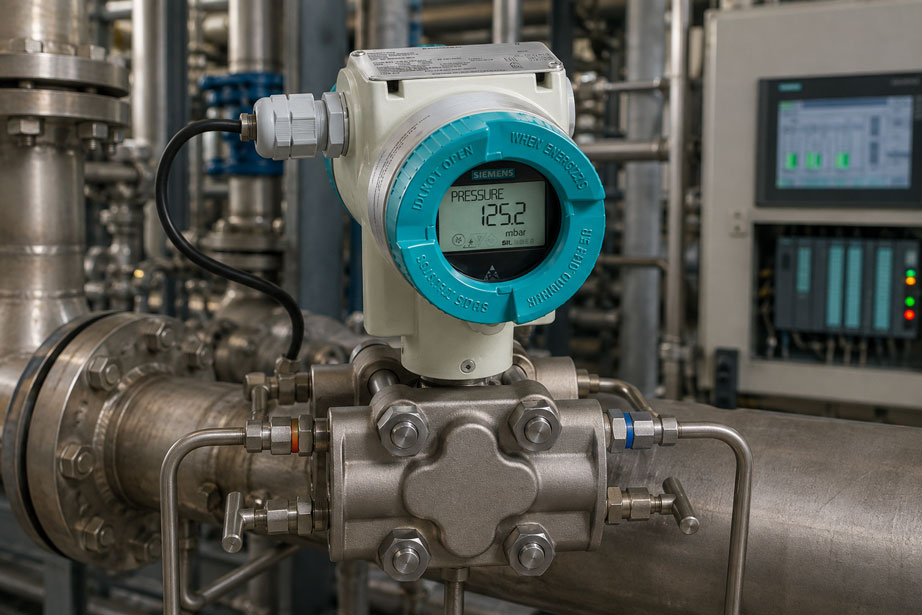
A differential pressure transmitter is configured for a measuring range of 0...100 mbar and transmits its measured value to a PLC using a 4...20 mA signal. At a measured differential pressure of 25 mbar, the visualization shows a flow rate of 25%. At first glance, this assignment seems logical: 25 mbar corresponds to 25% of the measuring range, so it might appear that the flow rate should also be 25%.
With a conventional differential-pressure flow measurement using an orifice plate, nozzle or Venturi tube, however, this assumption is normally incorrect. The generated differential pressure does not increase linearly with flow. In simplified form, Δp ∝ Q², and therefore Q ∝ √Δp. One quarter of the maximum differential pressure therefore already corresponds to one half of the maximum flow rate.
With a measuring range of 0…100 mbar, 25 mbar therefore represents not 25% but 50% of the maximum flow. If the electrical output of the measurement system is intended to be directly proportional to flow, the differential pressure must therefore be processed mathematically by applying a square root function.
This square root extraction can basically be performed at different points in the signal chain. An intelligent differential pressure transmitter can perform the square root function internally and then transmit a 4…20 mA signal that is linear to flow. Alternatively, the transmitter can output the differential pressure linearly and the PLC or process control system performs the square root calculation.
Both approaches work technically. The decisive requirement is that it is clearly documented which process variable the 4…20 mA signal actually represents. Particularly problematic are systems in which both the transmitter and the PLC apply square root extraction, or systems in which no square root function is applied at all. The 4 mA and 20 mA endpoints may still appear correct in both cases, while intermediate values can be significantly wrong.
In addition, the lower flow range is particularly sensitive because of the square root function. Even a small differential-pressure offset can produce a comparatively large apparent flow indication after square root extraction. Zero adjustment, low-flow cutoff and the correct design of the impulse lines are therefore just as much part of the measurement chain as the transmitter and PLC scaling.
For a correctly scaled differential-pressure flow measurement, one central question must therefore be answered clearly: Does the 4…20 mA signal represent linear differential pressure or already the square-rooted flow rate – and at which point in the signal chain is the square root applied exactly once?
Why Flow and Differential Pressure Are Not Linearly Related
In a conventional differential-pressure flow measurement, a defined restriction is introduced into a pipe, for example by an orifice plate, nozzle or Venturi tube. The restriction changes the local flow velocity and at the same time creates a pressure difference between two defined pressure tapping points.
This pressure difference is transmitted through impulse lines to the differential pressure transmitter. Under the process conditions used for the specific design, the simplified relationship is Δp ∝ Q². Differential pressure therefore increases with the square of the flow rate. Conversely, the flow rate is described by Q ∝ √Δp.
For normalized flow, the relationship can be simplified as Q / Qmax = √(Δp / Δpmax). This relationship explains why a 4…20 mA signal that is linear to differential pressure cannot simply be scaled linearly to a flow range.
If the flow rate increases from 50 to 100%, for example, the corresponding differential pressure increases fourfold from 25 to 100%. Conversely, halving the differential pressure does not mean halving the flow rate.
What Does Square Root Extraction Mean?
Square root extraction in this context simply means calculating the square root. The differential pressure measured by the transmitter is mathematically processed so that the resulting value is proportional to flow.
At 25% of the maximum differential pressure, for example, √0.25 = 0.5. This means that 50% of the maximum flow is already present. At 50% differential pressure, √0.50 ≈ 0.7071, corresponding to approximately 70.7% flow. Only at the upper end of the range do the percentage values match again: 100% differential pressure corresponds to 100% flow.
This non-linearity is not a fault of the differential pressure transmitter. It results from the physical measurement principle of the primary flow element and must therefore be taken into account during signal processing.
Option 1: Transmitter Outputs Linear Differential Pressure
The differential pressure transmitter can be configured so that its 4…20 mA output is linear to the measured differential pressure. With a range of 0...100 mbar, 0 mbar then corresponds exactly to 4 mA and 100 mbar exactly to 20 mA.
A differential pressure of 25 mbar therefore represents 25% of the configured span and generates an output current of 8 mA. However, this value still represents differential pressure. In terms of the flow measurement, the same 25 mbar already corresponds to 50% of the maximum flow.
The PLC must therefore first normalize the input current to the differential-pressure range, then calculate the square root and finally scale the result to the required flow range. The signal chain is therefore differential pressure → linear 4...20 mA signal → square root extraction in PLC → flow.
This configuration is particularly useful when the unprocessed differential pressure is also required as a separate process value or when the complete flow calculation is intentionally performed centrally in the control system.
Option 2: Transmitter Outputs Square-Rooted Flow
Many intelligent differential pressure transmitters can perform the square root function internally. The sensor continues to measure the actual differential pressure, but processes this value internally and generates a 4…20 mA signal that is linear to the calculated flow rate.
For a flow range of 0…1,000 m³/h, for example, 4 mA can represent 0 m³/h, 12 mA 500 m³/h and 20 mA 1,000 m³/h. The PLC can then scale this signal directly and linearly to the required flow unit.
The signal chain in this case is differential pressure → square root extraction in transmitter → linear 4...20 mA flow signal → PLC.
If the square root function is already enabled in the transmitter, the PLC must not apply a second square root function to the same measurement.
Comparing Linear and Square-Rooted 4…20 mA Signals
The difference between the two configurations becomes particularly clear when intermediate values rather than only the endpoints are considered.
| Differential Pressure | Corresponding Flow | 4…20 mA Linear to Δp | 4…20 mA Square-Rooted / Linear to Q |
|---|---|---|---|
| 0% | 0% | 4.00 mA | 4.00 mA |
| 6.25% | 25% | 5.00 mA | 8.00 mA |
| 25% | 50% | 8.00 mA | 12.00 mA |
| 50% | 70.71% | 12.00 mA | approx. 15.31 mA |
| 100% | 100% | 20.00 mA | 20.00 mA |
The table immediately shows why checking only 4 and 20 mA is insufficient. At both endpoints, the linear differential-pressure signal and the square-rooted flow signal are identical. The differences only become visible between the endpoints.
A functional test should therefore include at least one characteristic intermediate point. 25% differential pressure is particularly useful because, with correct square root extraction, it corresponds exactly to 50% flow.
Why 25% Differential Pressure Means 50% Flow
This relationship is particularly useful for a quick plausibility check of the measurement loop. For a flow rate of 50%, the reverse relationship is Δp = Q². Using a normalized flow value of 0.5 gives 0.5² = 0.25. Therefore, only 25% of the maximum designed differential pressure is required for half of the maximum flow.
With a differential-pressure range of 0…100 mbar, 25 mbar therefore corresponds to 50% flow. If the transmitter is configured for a square-rooted output characteristic, its current output at this point must be approximately 12 mA. If the output is linear to differential pressure, however, 8 mA is correct.
This single test point therefore already provides a very good indication of whether the output is configured as linear differential pressure or square-rooted flow.
Programming Square Root Extraction in the PLC Correctly
If the transmitter outputs differential pressure linearly, the 4…20 mA signal must first be normalized. For a standard range of 4…20 mA, this can be simplified as x = (I - 4 mA) / 16 mA. The normalized value x = 0 corresponds to the lower range value and x = 1 to the upper range value.
The normalized flow is then obtained by taking the square root. For the actual flow rate, the simplified relationship is Q = Qmax × √x.
With an input current of 8 mA, for example, x = (8 - 4) / 16 = 0.25. The square root is 0.5. With a maximum flow of 1,000 m³/h, the resulting flow rate is therefore 500 m³/h.
The sequence is important: normalize current signal → calculate square root → scale to flow. With offset ranges, special characteristics or bidirectional applications, this simplified calculation must not be used without verification.
Detecting Double Square Root Extraction
One of the most common configuration errors occurs when the transmitter already outputs a square-rooted flow signal while a square root function is also enabled in the PLC. The signal is then square-rooted twice.
Assume that the actual flow rate is 25%. A correctly square-rooting transmitter generates a linear flow signal of 8 mA. If the PLC then treats this value as a normalized 25% input and calculates the square root again, it obtains √0.25 = 0.5. The displayed value becomes 50%, even though the actual flow rate is only 25%.
At an actual flow rate of 50%, applying the square root a second time would produce approximately 70.7%. At the upper end of the measuring range, both characteristics meet again. This is why a system with double square root extraction can appear to scale perfectly at 100% while all important part-load values are incorrect.
What Happens If No Square Root Extraction Is Applied?
The opposite error occurs when the transmitter outputs differential pressure linearly and the PLC also scales the signal only linearly as flow. In this case, the required square root function is completely missing.
At an actual flow rate of 50%, only 25% of the maximum differential pressure is generated. A linear 0…100 mbar transmitter therefore outputs 8 mA. A PLC without square root extraction interprets these 8 mA as 25% of its scaled flow range and therefore displays only half of the actual flow.
This error also disappears at 0 and 100%. A pure endpoint test can therefore miss it just as easily as double square root extraction.
Testing and Calibrating a Square-Rooted Transmitter Correctly
Before testing a differential pressure transmitter, it must be clearly known which process variable its analog output represents. With a device configured for 0…100 mbar differential pressure and 4…20 mA, the expected intermediate values differ completely depending on the configured characteristic.
| Applied Pressure | Differential Pressure | Expected Output with Linear Δp Characteristic | Corresponding Flow | Expected Output with Square-Rooted Characteristic |
|---|---|---|---|---|
| 0 mbar | 0% | 4.00 mA | 0% | 4.00 mA |
| 6.25 mbar | 6.25% | 5.00 mA | 25% | 8.00 mA |
| 25 mbar | 25% | 8.00 mA | 50% | 12.00 mA |
| 50 mbar | 50% | 12.00 mA | 70.71% | approx. 15.31 mA |
| 100 mbar | 100% | 20.00 mA | 100% | 20.00 mA |
A technician who automatically expects 12 mA at 50 mbar from every 0…100 mbar transmitter would therefore incorrectly classify a correctly square-rooted transmitter as faulty. Conversely, expecting 12 mA at 25 mbar would be incorrect for an output that is linear to differential pressure.
Before every calibration, it must therefore be clarified whether the analog output represents the actual differential pressure or already the calculated flow rate.
Why the Lower Flow Range Is Critical
The square root function is particularly sensitive to small differential-pressure changes close to zero. Zero errors, measurement noise, pressure pulsations or small hydrostatic differences therefore become much more significant in the lower measuring range.
| Differential Pressure | Theoretical Flow | Practical Significance |
|---|---|---|
| 0.25% | 5% | very small Δp values already produce visible flow indications |
| 1% | 10% | a small zero offset can become clearly visible |
| 6.25% | 25% | typical test point in the lower range |
| 25% | 50% | particularly useful plausibility test point |
| 50% | 70.71% | clear difference between Δp and Q scaling |
| 100% | 100% | both characteristics meet at the upper endpoint |
A differential-pressure offset of only 1% of the span would theoretically already produce 10% flow. The problem is therefore not necessarily caused by an inaccurate sensor cell, but also by the mathematical effect of the square root function on very small differential-pressure values.
Particularly in the lower range, zero stability, process stability and impulse-line conditions must therefore be considered carefully.
Setting the Low-Flow Cutoff Correctly
To prevent an unstable or physically meaningless flow indication close to zero, many transmitters and flow calculations include a low-flow cutoff. Below a defined threshold, the calculated flow is set to zero.
This prevents a small differential-pressure offset, noise or minor process pulsations from being displayed as actual flow or possibly even being integrated by a totalizer.
The threshold must not be selected arbitrarily high, however. A low-flow cutoff that is too high suppresses genuine low flow. If it is set too low, zero noise and drift can continue to produce an unwanted flow indication.
The appropriate setting therefore depends, among other things, on the design of the primary flow element, maximum differential pressure, required turndown, transmitter accuracy, process dynamics and the lowest flow rate that still needs to be measured reliably.
Zero Errors and Incorrect Flow Indication
The high sensitivity of the lower range explains why a correct zero point is particularly important in differential-pressure flow measurement. If a transmitter measures, for example, 1% differential pressure at an actually stationary process because of an offset, the square root function gives √0.01 = 0.10, corresponding theoretically to 10% flow.
Before adjusting the low-flow cutoff, it should therefore first be verified whether the measuring point has a stable physical zero. An incorrectly zeroed transmitter, unsuitable mounting position or different hydrostatic heads in the two impulse lines can create or simulate an actual differential pressure.
For liquid measurement, the impulse lines must be correctly filled according to the application. In steam applications, the intended condensate arrangement and defined liquid columns are important. A low-flow cutoff should not simply be used to hide such installation problems.
Considering Density Changes in Gases and Steam
The simplified relationship Q ∝ √Δp assumes that the other process variables relevant to the design remain sufficiently constant or are already taken into account. More generally, the relationship for a differential-pressure primary element can be approximated as Q ∝ √(Δp / ρ).
Density ρ is therefore another important influencing variable. For liquids with relatively stable density, a simple differential-pressure flow measurement may be sufficient for many applications. For gases and steam, however, density can change significantly with process pressure, temperature and, where relevant, composition.
If an accurate standard volumetric or mass flow is required under such conditions, additional pressure and temperature measurements or appropriate process compensation may therefore be necessary.
The square root function only establishes the fundamental relationship between differential pressure and flow. It does not compensate for relevant changes in gas or steam density.
Considering Bidirectional Flow Separately
The simple square root function is normally considered for positive differential pressure and therefore a defined flow direction. In systems where the flow direction can reverse, the measured differential pressure can also change sign.
An equation such as Q = √Δp is not sufficient for such an application. The direction must also be taken into account, for example in a form such as Q ∝ sign(Δp) × √|Δp|.
Whether such bidirectional measurement is supported by the primary element, differential pressure transmitter and control system must be checked for the specific measuring point. A conventional 0…100% configuration for only one flow direction must not be transferred without verification.
Systematically Troubleshooting the Signal Chain
If the displayed flow value is implausible, the PLC scaling or transmitter configuration should not be changed immediately. It is more effective to examine the entire signal chain from the actual generation of the differential pressure through to the visualization: primary flow element → impulse lines → differential pressure transmitter → 4...20 mA → analog input → PLC scaling → display.
| Observation | Possible Cause | Check |
|---|---|---|
| 25% Δp is displayed as 25% Q | square root extraction missing | check transmitter and PLC characteristics |
| 25% actual Q is displayed as 50% | double square root extraction | check whether transmitter and PLC both apply square root extraction |
| 0 and 100% correct, intermediate values wrong | incorrect characteristic or scaling | test 25% and 50% intermediate points |
| Flow indicated while process is stopped | zero offset or low-flow setting | check physical and electrical Δp zero |
| Display unstable near zero | Δp noise, pulsation or square-root amplification | investigate raw differential pressure and cutoff |
| Gas-flow indication changes with process pressure or temperature | density change not compensated | check pressure, temperature and compensation concept |
| Transmitter current plausible, PLC value incorrect | analog input or PLC scaling | compare current signal and raw input value |
Intermediate points are particularly informative. If only the lower and upper range values are tested, both missing and double square root extraction can remain completely hidden.
Practical Example: 0…100 mbar and 0…1,000 m³/h
An orifice plate is designed so that a differential pressure of 100 mbar is generated at a maximum flow of 1,000 m³/h. The connected differential pressure transmitter has a 4…20 mA output.
In the first case, the square root function is enabled in the transmitter. At an actual differential pressure of 25 mbar, the device calculates Q = 1,000 × √(25 / 100). This gives 500 m³/h. Because the analog output is already linear to flow, the transmitter outputs 12 mA. The PLC is simply scaled linearly with 4 mA = 0 m³/h and 20 mA = 1,000 m³/h.
In the second case, the transmitter outputs differential pressure linearly. At 25 mbar, its output is therefore only 8 mA. The PLC interprets this as a normalized differential-pressure value of 25%, calculates √0.25 = 0.5 and again correctly determines 500 m³/h.
Both concepts therefore produce the same correct result. The only difference is where the square root function is performed.
The third case is problematic: The transmitter already outputs the square-rooted 12 mA corresponding to 50% flow, while the PLC applies the square root once again to the normalized 50% value. From √0.5 ≈ 0.707, the system incorrectly displays approximately 707 m³/h. The actual flow remains only 500 m³/h.
The error at this operating point is therefore more than 40% of the actual flow value, even though both the lower and upper endpoints of the measuring range may appear to function correctly.
Commissioning Step by Step
- Check the design data and type of the primary differential-pressure flow element.
- Determine the maximum differential pressure at the specified maximum flow.
- Check the measuring range and configuration of the differential pressure transmitter.
- Define and document whether square root extraction will be performed in the transmitter or in the control system.
- Verify whether the 4…20 mA output actually represents differential pressure or already represents flow.
- Match the PLC scaling exactly to this transmitter configuration.
- Ensure that exactly one square root function is active in the complete signal chain.
- Check the zero point of the differential pressure transmitter under correct process or test conditions.
- Set the low-flow cutoff according to the measurement task.
- Check the lower and upper electrical or pneumatic range points.
- Test at least one characteristic intermediate point; 25% differential pressure corresponding to 50% flow is particularly useful.
- For gas or steam applications, check whether pressure or temperature compensation is required.
- Clearly document units, ranges, characteristic function and process variable in the transmitter, PLC and visualization.
Common Mistakes
- Scaling differential pressure directly as flow: The required square root function is missing.
- Transmitter and PLC both apply square root extraction: The signal is processed twice with the square root function.
- Checking only 4 and 20 mA: An incorrect characteristic remains undetected at both endpoints.
- Assuming 25% differential pressure equals 25% flow: In reality, 25% Δp corresponds to 50% Q.
- Assuming 50% differential pressure equals 50% flow: In reality, 50% Δp corresponds to approximately 70.7% Q.
- Calibrating a square-rooted transmitter like a linear pressure transmitter: The expected intermediate values are calculated incorrectly.
- Setting the low-flow cutoff too high: Genuine low flow is suppressed.
- Setting the low-flow cutoff too low: Zero drift and noise may continue to appear as flow.
- Ignoring zero errors: Because of the square root function, even a small Δp offset can produce a significant flow indication.
- Ignoring gas density: Square root extraction alone does not compensate for relevant pressure and temperature changes.
- Using an incorrect maximum differential pressure: The transmitter range and the design of the primary element no longer match.
- Failing to document the process variable: It later becomes unclear whether 4…20 mA represents differential pressure or already the calculated flow.
Suitable Differential Pressure Transmitter
For industrial differential-pressure and differential-pressure flow measurements, the Siemens SITRANS P320, for example, is suitable. The digital process pressure transmitter can be used for differential-pressure measurement as well as applications such as volumetric flow, mass flow or level measurement based on differential pressure.
For differential-pressure flow applications, a square-rooted output characteristic can be used. The transmitter measures the differential pressure and processes it so that the analog output subsequently represents a value proportional to flow. The downstream control system can therefore scale the 4…20 mA value directly and linearly to the required flow unit.
Depending on the configuration, functions for the lower flow range or low-flow suppression are also available. HART communication additionally allows configuration and diagnostics using suitable communication or engineering tools.
For particularly demanding applications, the SITRANS P420 is also available within the same product family.
Further differential pressure transmitters, pressure transmitters and accessories for industrial process measurement can be found under Pressure Measurement Technology at ICS Schneider.
Further fundamentals on the linear assignment of a 4…20 mA signal can be found in the article Scaling a 4–20 mA Digital Display: Displaying the Process Value Correctly.
Conclusion
In a conventional differential-pressure flow measurement, the generated differential pressure is not linear to the actual flow. In simplified form, Δp ∝ Q² and therefore Q ∝ √Δp. A square root function must therefore be present somewhere in the signal chain.
If the differential pressure transmitter outputs its measured value linearly as a Δp signal, square root extraction must be performed in the PLC or process control system. If the square root function is already enabled in the transmitter, its 4…20 mA output represents flow and the PLC must then scale the signal only linearly.
Checking intermediate values is particularly important. 25% differential pressure already corresponds to 50% flow, while 50% differential pressure corresponds to approximately 70.7% flow. Since both characteristics have the same values at 0 and 100%, a pure endpoint test can miss both missing and double square root extraction.
In the lower range, the square root function also increases the effect of very small differential-pressure values. An offset of only 1% of the Δp span theoretically already corresponds to 10% flow. A stable zero point and a suitably selected low-flow cutoff are therefore especially important.
Gas and steam measurements involve another influence. If density changes significantly because of process pressure or temperature, the square root function alone may not be sufficient for accurate standard volumetric or mass-flow measurement. Additional process variables may then have to be included.
The most important question during commissioning, troubleshooting and calibration is therefore: Do the 4…20 mA currently represent linear differential pressure or already the calculated flow – and is the square root really applied exactly once in the complete signal chain?
FAQ: Square Root Extraction for Differential-Pressure Flow
Why must a differential-pressure signal be square-rooted for flow measurement?
With conventional differential-pressure primary elements, the generated differential pressure is approximately proportional to the square of the flow rate. To obtain a value proportional to flow from the differential pressure, the square root must therefore be calculated.
How much flow corresponds to 25% differential pressure?
25% differential pressure corresponds to 50% flow because √0.25 = 0.5. With a maximum flow of 1,000 m³/h, 25% differential pressure therefore corresponds to 500 m³/h.
How much flow corresponds to 50% differential pressure?
The square root of 0.5 is approximately 0.7071. Therefore, 50% differential pressure corresponds to approximately 70.7% of the maximum flow.
Should square root extraction be performed in the transmitter or in the PLC?
Both approaches are generally possible. The important point is that the square root function is applied at only one point in the signal chain. If the transmitter outputs linear differential pressure, the PLC must apply square root extraction. If the transmitter already outputs a signal linear to flow, the PLC must only apply linear scaling.
How can I determine whether my differential pressure transmitter already applies square root extraction?
A suitable intermediate point quickly provides the answer. With a range of 0…100 mbar, for example, apply 25 mbar. A linear differential-pressure output produces 8 mA. A square-rooted flow output produces 12 mA.
What happens with double square root extraction?
The flow is displayed significantly too high in the partial-load range. At an actual flow of 25%, for example, a second square root function would produce an indication of 50%. The error disappears again at the lower and upper endpoints.
What happens if no square root extraction is applied?
The flow is displayed significantly too low in the partial-load range. At 50% actual flow, only 25% of the maximum differential pressure is generated. Purely linear scaling would therefore incorrectly indicate only 25% flow.
What is a low-flow cutoff?
A low-flow cutoff sets very small calculated flow values below a defined threshold to zero. This is intended to prevent zero drift, differential-pressure noise or minor pulsations from being interpreted as actual flow.
Why is the flow indication often unstable near zero?
The square root function is highly sensitive in the lower differential-pressure range. Just 1% differential pressure theoretically corresponds to 10% flow. Small zero shifts or process fluctuations can therefore become clearly visible.
How do I test a square-rooted 4…20 mA transmitter?
The expected output values must be calculated according to the square root function. With a range of 0…100 mbar, for example, 25 mbar produces 12 mA with a square-rooted output, while 50 mbar produces approximately 15.31 mA.
Is square root extraction sufficient for accurate gas-flow measurement?
Not always. With gases, differential-pressure flow also depends on density. If process pressure or temperature changes significantly, additional pressure and temperature compensation may be required.
Can bidirectional flow also be measured using differential pressure?
In principle, yes, provided that a suitable primary flow element, differential pressure transmitter and evaluation concept are used. However, the simple positive square root function is not sufficient because the sign of the differential pressure and therefore the direction of flow must also be taken into account.