Condensing Measurement Data at the Edge: Combining Average, Minimum, Maximum and Raw Data Effectively

→ Product category: IIoT solutions

 

A sensor supplies one measured value every second. With 100 measuring points, this already produces 8.64 million values per day – even before timestamps, quality information, protocol overhead, database indexes or backups are taken into account. If all raw data is transmitted permanently to a central platform, bandwidth requirements, storage demand and costs increase rapidly.

Simply reducing the data to hourly or daily averages only appears to solve the problem. Short pressure peaks, temperature drops, starting currents or vibrations can disappear completely, even though they may be crucial for maintenance and troubleshooting. Effective data aggregation must therefore reduce data volumes without destroying information that is operationally important.

This article explains how to combine sampling rate, time windows, average, minimum, maximum, event data and selected raw data. It also describes which time and quality information belongs to each aggregate and how to build a data strategy that supports both dashboards and subsequent root-cause analysis.

Table of Contents

1. Separating sampling, processing, transmission and storage
2. Defining the evaluation objective before aggregation
3. Defining time windows unambiguously
4. Calculating and interpreting averages correctly
5. Using minimum and maximum to preserve peaks
6. Adding count, start, end and dispersion
7. Retaining selected raw data instead of discarding it completely
8. Using event-triggered raw data and ring buffers
9. Managing timestamps and clock synchronisation
10. Keeping data quality and missing values visible
11. Estimating storage requirements and the reduction factor
12. Planning multi-tier retention
13. Distributing tasks between sensor, edge and cloud
14. Considering MQTT, OPC UA and the data model together
15. Practical example: aggregating a plant pressure profile
16. Recommended implementation procedure
17. Common data aggregation mistakes
18. Suitable IIoT products from ICS Schneider
19. Conclusion
20. FAQ: Aggregating measurement data at the edge

Separating Sampling, Processing, Transmission and Storage

Several time-related concepts are frequently mixed together in IIoT projects. For a reliable data architecture, four levels should be considered separately:

• Sampling rate: How often does the sensor or input module acquire the physical measured value?
• Processing rate: How often does the local logic evaluate new values, update aggregates or check limits?
• Transmission rate: How often does the field device or gateway send data to the higher-level system?
• Storage rate: Which values are actually stored permanently in the local or central database?

For example, a device may measure every second and check a limit every second, but transmit a data packet only once every five minutes. This does not automatically mean that the values between transmissions are lost. Depending on the device, they may be processed locally, buffered or combined into aggregates. These functions must, however, be verified for the specific product; the description “IIoT-enabled” alone guarantees neither average calculation nor raw-data storage.

This distinction is also important for troubleshooting. A smoothed trend may result from a low sensor sampling rate, a device filter, slow transmission or subsequent database aggregation. Without a documented processing chain, it is no longer possible to determine where information was lost.

Defining the Evaluation Objective Before Aggregation

The appropriate aggregation strategy is determined not by the available storage but by the later question to be answered. Typical objectives differ considerably:

• For energy and quantity balances, time-weighted averages, meter readings or integrals are crucial.
• For limit monitoring, minimum, maximum and the duration of limit violations must be retained.
• For condition monitoring, dispersion, rate of change, frequency components or event features are relevant.
• For root-cause analyses, raw data from before, during and after an event is required.
• For management dashboards, longer time windows and more highly aggregated metrics are often sufficient.

A single data stream cannot satisfy every requirement optimally. A combination of permanently stored aggregates, raw data available for a limited period and event-related raw-data blocks is therefore usually more robust than choosing either “store everything” or “store averages only”.

Defining Time Windows Unambiguously

Every aggregate relates to a time window. This window must be defined unambiguously. For regular reporting, non-overlapping consecutive windows – for example, every full minute – are usually the simplest:

[10:00:00, 10:01:00), [10:01:00, 10:02:00), …

This notation means that the start time belongs to the window, while the end time already belongs to the next window. This prevents any measured value from being counted twice. The time zone, UTC reference and handling of incomplete windows must also be defined.

Overlapping sliding windows are suitable for continuous condition assessments, but they produce more strongly interdependent results and more data. A sliding 15-minute average recalculated every minute consists of 15 minutes of data but provides a new value every minute. Fixed windows are generally more transparent for archiving and accounting, while a sliding window can be useful for online monitoring.

Each record must include at least the window start, window end and aggregation method used. A timestamp of “10:01” without a clear definition leaves open whether it refers to the start, end or midpoint of the window.

Calculating and Interpreting Averages Correctly

With a constant sampling interval, the arithmetic mean can be used:

Average = sum of valid measured values / number of valid measured values

With irregular intervals, a simple average can distort the result. A time-weighted average is then more appropriate:

Time-weighted average = Σ(measured value × valid duration) / Σ(valid duration)

The average describes the mean level within the window. However, it contains no information about whether the process was steady or fluctuated between large excursions. A simple example illustrates the consequences:

• 60 values constantly at 5 bar produce an average of 5 bar.
• 30 values at 0 bar and 30 values at 10 bar also produce an average of 5 bar.

The two processes are operationally completely different. The average should therefore be combined at least with the minimum and maximum. For dynamic applications, standard deviation, range or limit-violation duration can also be useful.

Using Minimum and Maximum to Preserve Peaks

Minimum and maximum preserve the magnitude of the extreme values acquired within a window. They prevent a short peak from disappearing completely in the average. Correct interpretation nevertheless requires additional information:

• time of the minimum and maximum,
• quality status of the underlying raw values,
• number of identical extreme values, where relevant,
• sampling rate and upstream filtering.

A maximum preserves only the magnitude of a peak, not its shape or duration. A single measured value of 12 bar and a load of 12 bar lasting 40 seconds can produce the same maximum in a one-minute aggregate. Limit assessments should therefore also retain the duration above the limit, the number of violations or an event record.

Minimum and maximum can only retain peaks that were sampled in the first place. A pressure surge lasting 20 milliseconds may remain completely invisible when sampling once per second. Data aggregation therefore begins only after signal acquisition and filtering have been selected appropriately for the application.

Adding Count, Start, End and Dispersion

For a meaningful aggregate, four values are often a sensible minimum:

Average + minimum + maximum + number of valid values

The count indicates whether the window is complete. If only 42 rather than 60 valid values are processed with an expected one-second sampling interval, an average can still be calculated but cannot readily be compared with a complete window.

Depending on the application, the following metrics can be added:

• Start and end values: Preserve the direction of change and allow a simple difference to be calculated.
• Standard deviation: Describes dispersion without storing the complete signal shape.
• Range: Difference between maximum and minimum.
• Limit duration: Time above or below a defined limit.
• Number of state changes: Useful for switches, pumps or valves.
• Quality proportions: Percentage of valid, uncertain or faulty input values.

The metrics to be stored should be defined for each measured quantity. Average, minimum and maximum may be sufficient for a slowly changing room temperature. Additional event and dispersion values may be required for pump pressure or machine current.

Retaining Selected Raw Data Instead of Discarding It Completely

Aggregates cannot be converted back into the original raw data. Once the sequence and intermediate values have been deleted, subsequent analyses are limited to the stored metrics. Before deletion, it should therefore be determined which currently unknown questions may arise in the future.

A robust strategy combines three data classes:

• Short-term raw data: Complete high-resolution data for several days or weeks.
• Long-term aggregates: Average, minimum, maximum, count and quality information for months or years.
• Event raw data: High-resolution data blocks around alarms, shutdowns, maintenance activities or unusual changes.

This keeps recent faults available for detailed investigation while long-term trends remain accessible with significantly lower storage requirements. Raw data can be retained for longer at particularly important measuring points than for purely comfort-related or environmental values.

Using Event-Triggered Raw Data and Ring Buffers

If an event is detected only after it occurs, the immediately preceding values are often the most valuable for root-cause analysis. A local ring buffer therefore continuously stores the most recent minutes or hours. When a trigger occurs, the relevant period preceding the event is saved and supplemented by a defined post-trigger period.

Possible triggers include:

• exceeding or falling below a limit,
• an unusually rapid change,
• a large range or standard deviation within a short window,
• a machine state change,
• a communication failure or poor signal quality,
• manual marking by service personnel.

Triggers require hysteresis, a minimum duration and, where applicable, a lockout period so that a noisy signal does not create countless events. It must also be defined how simultaneous or overlapping events are combined.

Managing Timestamps and Clock Synchronisation

A measurement series can only be evaluated across different systems if its time reference is reliable. Ideally, several times are distinguished:

• Source time: Time at which the sensor or controller acquired the value.
• Edge arrival time: Time at which the gateway received the value.
• Transmission or storage time: Time of transmission or database ingestion.

Source time is generally decisive for process analyses. Arrival and storage times help identify communication delays, buffering and data transmitted retrospectively. All clocks involved must be synchronised using a suitable time source; the required accuracy depends on the process dynamics.

Late-arriving data must be considered during aggregation. A one-minute window must not silently receive different values retrospectively without versioning or identification. A defined lateness allowance, a status for incomplete windows and clear rules for values arriving later are advisable.

Keeping Data Quality and Missing Values Visible

An average calculated from 60 good measured values is not equivalent to an average calculated from ten uncertain values and 50 communication gaps. Quality information must therefore not be lost during aggregation.

At least the following should be stored with each aggregate:

• number of expected and actually used values,
• number or proportion of invalid and uncertain values,
• “complete” or “partial window” status,
• information on whether values were interpolated or substituted,
• device and communication status, where available.

Missing values must not automatically be interpreted as zero. Likewise, an invalid extreme value should not appear as the minimum or maximum without a defined rule. The OPC UA aggregate models demonstrate how closely an aggregate, its time window and quality status are linked: in addition to functions such as minimum and maximum, quality and partial-window states are also described.

Estimating Storage Requirements and the Reduction Factor

The number of raw values per day can be estimated easily:

Raw values per day = number of sensors × sampling rate × 86,400

With 100 sensors and one sample per second, 8.64 million raw values are produced every day. If, as an example, 32 bytes per logical record are assumed for value, timestamp, identifier and status, this amounts to approximately 276 MB per day – excluding database overhead, indexes, replication and backups.

If average, minimum, maximum and count are stored for each sensor and minute, this produces:

100 sensors × 1,440 minutes × 4 values = 576,000 aggregate values per day

Four metrics are stored instead of 60 raw values per minute. In this example, the number of values is therefore reduced by a factor of 15. If the times of the extreme values, quality proportions and event data are also stored, the reduction is smaller – but the information value increases considerably.

For realistic capacity planning, the message and database formats, compression, metadata, indexes, replication, backups, retention period and expected event rate must be included.

Planning Multi-Tier Retention

Instead of deleting all data after the same period, a multi-tier retention strategy is recommended. One possible concept is:

Data tier	Example resolution	Example retention period	Main purpose
Raw data	1 second	14 days	current troubleshooting
Short-term aggregates	1 minute	12 months	operations and maintenance
Long-term aggregates	15 minutes or 1 hour	several years	trends, reports and planning
Event data	high resolution with pre- and post-trigger data	according to criticality	root-cause analysis and evidence

These periods are not universally applicable. They must match the process risk, warranty obligations, regulatory requirements, analysis needs and storage budget. Before any automatic deletion, it should be verified that the aggregates have already been generated completely and traceably.

Distributing Tasks Between Sensor, Edge and Cloud

Aggregation at the edge reduces transmission volume and continues to operate when connectivity is limited. At the same time, local processing must not become an opaque black box. An appropriate distribution of tasks may look as follows:

• Sensor or measuring instrument: Physical acquisition, necessary signal filtering, status information and, where applicable, local limit checking.
• Edge device or gateway: Time reference, protocol conversion, window aggregation, ring buffer, event detection and store-and-forward.
• Central platform: Long-term storage, cross-site analysis, visualisation, model creation and management of data rules.

The configuration of the edge logic must be versioned. If a time window changes from one minute to five minutes or a filter time is adjusted, data from before and after the change is not comparable without appropriate identification. The configuration version and calculation rule therefore belong in the data model.

Considering MQTT, OPC UA and the Data Model Together

A communication protocol does not automatically resolve the semantic issues of aggregation. MQTT transports messages but does not define the application-specific payload model. The project must therefore define whether a value is a raw value, average or maximum, which window it relates to and which quality status it has.

An aggregate record should contain at least:

• unique measuring-point identifier,
• measured quantity and unit,
• window start and window end,
• aggregation function,
• value and, where applicable, time of the extreme value,
• sample count and quality information,
• version of the calculation and device configuration.

OPC UA describes standardised aggregate functions and quality states, including average, minimum, maximum, count and the times of extreme values. Nevertheless, it is essential to establish which functions the specific device, server or platform actually supports and how they are configured.

For wireless and LPWAN systems, a distinction must also be made between measurement and transmission intervals. A device may measure more frequently than it transmits data packets. This saves energy and wireless data volume but requires clear rules governing which information is included in the packet and what happens if the connection is interrupted.

Practical Example: Aggregating a Plant Pressure Profile

A pressure measuring point is sampled every second. One-minute values are to be transmitted for the operational dashboard, but short pressure peaks must remain identifiable for maintenance.

For every full one-minute window, the edge system stores:

• time-weighted average,
• minimum with timestamp,
• maximum with timestamp,
• start and end values,
• number of valid and invalid measured values,
• time above the warning threshold.

At the same time, a ring buffer retains the raw data from the preceding ten minutes. If the pressure exceeds 8 bar or rises by more than 1 bar within two seconds, five minutes before and five minutes after the trigger are saved as an event record.

In one example minute, 59 values are close to 5 bar and one value is 9 bar. The average is only approximately 5.07 bar and would appear inconspicuous in the trend. The maximum of 9 bar reveals the peak. The time of the maximum allows it to be assigned to a switching operation, while the retained raw-data block shows the shape, duration and preceding history of the peak.

If communication with the central platform fails, aggregates and event data are buffered locally and transmitted later with their original source time. The arrival time in the cloud does not replace the measurement time.

Recommended Implementation Procedure

1. Describe the measurement task: Clearly identify the operational decision, alarm, evidence and subsequent analysis.
2. Determine the process dynamics: Define the shortest relevant event duration and required sampling rate.
3. Document the signal path: Record sensor filters, PLC cycle, gateway polling and platform processing.
4. Define the windows: Specify their duration, alignment, time zone and behaviour at window boundaries.
5. Select the aggregates: Determine the average, minimum, maximum, count and application-specific supplementary values.
6. Define quality rules: Specify how invalid, uncertain, missing and interpolated values are handled.
7. Plan the raw-data strategy: Define short-term retention, ring buffers and pre- and post-trigger periods.
8. Configure events: Specify limits, rates of change, hysteresis and lockout periods.
9. Synchronise time: Document source time, arrival time, UTC reference and permitted deviation.
10. Protect transmission: Verify buffering, retransmission and duplicate detection in the event of connection failures.
11. Version the data model: Include the calculation method, units and configuration version.
12. Test with real events: Simulate peaks, outages, late data and device replacements.
13. Measure storage demand: Use the actual record size and event rate rather than theoretical values alone.
14. Review regularly: Adapt aggregation rules to new analysis and operational requirements.

Common Data Aggregation Mistakes

Mistake	Typical consequence	Better approach
Storing averages only	Short extreme values and fluctuations disappear	Add at least minimum, maximum and count
Treating sampling and transmission intervals as identical	The actual measurement resolution remains unclear	Document all processing levels separately
Storing the maximum without its timestamp	It cannot be assigned to plant events	Retain the time of the extreme value
Treating missing values as zero	The average and minimum are distorted	Identify missing values and store the count
Calculating an arithmetic mean from irregularly spaced values	Long-lasting states are weighted incorrectly	Use a time-weighted average
Deleting raw data immediately	Subsequent root-cause analysis is no longer possible	Provide short-term raw data and an event buffer
No clock synchronisation	Events from different systems do not align in time	Define a suitable time source and permitted deviation
Aggregation without quality status	Complete and incomplete windows appear equivalent	Store quality proportions and partial-window status
Changing the configuration without identification	Historical time series become incomparable	Store the calculation rule and version with the data

Suitable IIoT Products from ICS Schneider

WIKA PEW-1000 – Measure Frequently and Transmit as Required

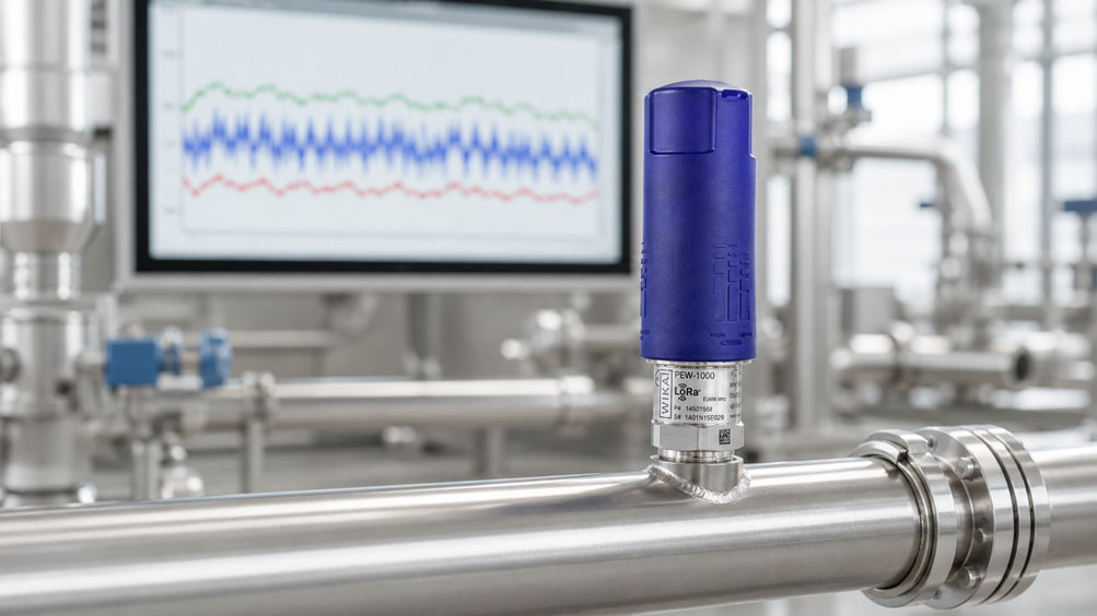
The WIKA PEW-1000 is a wireless pressure sensor for industrial applications. Measurement and transmission intervals can be configured depending on the measured value. The instrument can measure more frequently without transmitting every single measured value. It therefore illustrates particularly well the fundamental difference between local acquisition and wireless transmission.

Which measured values, status information and aggregation functions are transmitted or processed in the platform for a specific configuration must be defined based on the device and system configuration.

WIKA NETRIS®2 – Transmit Two 4…20 mA Signals via LoRaWAN®

The WIKA NETRIS®2 radio unit acquires two intrinsically safe analogue 4…20 mA input signals and transmits the measured data to a cloud in configurable LoRaWAN® data packets. It is suitable for remote monitoring and preventive maintenance in hazardous areas.

WIKA NETRIS®3 – Integrate Digital Instrument Data into the IIoT Structure

The WIKA NETRIS®3 radio unit receives data digitally from a compatible WIKA measuring instrument and transmits it to a cloud in configurable data packets via LoRaWAN®. It is designed for centralised remote monitoring and big-data applications in the process industry.

WIKA A2G-500 – Decentralised Data Node for Building Services

The WIKA A2G-500 measures differential pressure, gauge pressure and vacuum in ventilation and air-conditioning systems. Measured values are available as analogue signals, via Modbus® RTU or LoRaWAN®. Depending on the version, the device can integrate up to four input signals as a decentralised data node.

Further wireless measuring instruments and solutions for digital pressure, temperature and level monitoring can be found in the IIoT Solutions category at ICS Schneider.

Conclusion

Effective edge aggregation reduces data volume without unnecessarily destroying operational information. The average describes the level, while minimum and maximum preserve acquired extreme values. Count and quality status indicate how reliable the result is. The times of extreme values, limit duration and dispersion metrics supplement the information depending on the application.

Raw data nevertheless remains indispensable when the signal shape, sequence of events or previously unknown relationships need to be investigated. A practical architecture therefore combines short-term raw data, long-term aggregates and high-resolution event data from a ring buffer.

Clearly defined time windows, synchronised clocks, traceable quality rules and versioned calculations are essential. Only when sampling, processing, transmission and storage are documented separately will measurement data remain reliably interpretable months or years later.

FAQ: Aggregating Measurement Data at the Edge

Which values should an edge device store as a minimum?

For many process variables, average, minimum, maximum, number of valid values, window start, window end and quality status represent a sensible minimum. The exact selection depends on the process dynamics and evaluation objective.

Are minimum and maximum sufficient to preserve peaks?

They preserve the magnitude of a sampled extreme value, but not its shape and duration. For critical peaks, the timestamp, limit duration and a raw-data block around the event should also be stored.

When is a time-weighted average required?

When measured values arrive at irregular intervals or remain valid for different lengths of time. With a constant sampling interval, the time-weighted average will generally equal the arithmetic mean.

How long should an aggregation window be?

The window must be significantly shorter than the relevant process changes and must match the operational decision. One minute may be sufficient for slowly changing temperature profiles but much too long for pressure surges or vibrations.

Should raw data be deleted completely?

Not immediately. Limited short-term retention and event-triggered raw-data blocks preserve the possibility of root-cause analysis without requiring all raw values to be stored permanently.

What happens if the connection is interrupted?

The edge system should buffer data locally and transmit it later with the original source time. Buffer capacity, overflow behaviour, retransmission and duplicate detection must be defined and tested.

Is MQTT already a form of data aggregation?

No. MQTT is a transport protocol. The payload model must define which raw values or aggregates are transmitted and how time windows, quality and units are described.

What role does OPC UA play in aggregates?

OPC UA defines standardised aggregate functions and associated quality information. Whether a specific server or device supports these functions must, however, be checked against its implementation and configuration.

Why should the sample count be stored?

It shows whether the time window is complete and how many values were actually included in the calculation. Without a count, a complete average and a severely incomplete average can look identical.

Can edge aggregation compensate for a sampling rate that is too low?

No. A peak that was not acquired cannot be reconstructed later. The sampling rate must first be appropriate for the process dynamics; only then should the data be aggregated.