


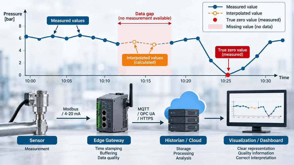
A pressure sensor sends one measured value per minute to an edge gateway. In the historian, the time series initially looks clean: 6.21 bar, 6.18 bar, 6.24 bar. Then three minutes of data are missing. The recording subsequently continues at 6.27 bar.
What should now be stored for those three missing minutes?
At first glance, the options appear similar. You could enter 0. You could continue using the last known value. You could interpolate between 6.24 and 6.27 bar. Or you could simply leave the positions empty.
For later analysis, however, these options are completely different.
A value of 0 bar is a measured value. It can, for example, mean that a system was depressurised. A missing measured value, by contrast, means that no reliable measurement information is available for the relevant time. An interpolated value is a calculated estimate between known data points. It can be useful for a trend, but it is not an actually measured raw value.
If these states are treated identically in the database, the meaning of the time series is changed without anyone noticing. Average values become distorted, machine shutdowns appear to have occurred even though only communication failed, and calculated replacement values may later be mistaken for original measurements.
Especially in IIoT architectures, the problem does not arise only in the database. A measurement often passes through several layers: sensor, PLC or fieldbus, edge gateway, local buffer, MQTT or OPC UA communication, broker, historian and finally dashboard or analytics platform. At each of these points, a value can arrive late, be discarded, duplicated or modified.
The most important rule is therefore: The numerical value alone is not sufficient for an industrial time series. A reliable data point requires at least an unambiguous time reference and information indicating whether the value was actually measured, invalid, missing, transmitted late or generated by calculation.
Why a data gap is not automatically a zero value
In many data projects, the problem begins with a seemingly harmless decision. A dashboard expects one numerical value for every minute. However, no data record is available for 10:15. To prevent the curve from showing a gap, software automatically inserts 0.
From a visualisation perspective, the time series is now complete. From a measurement perspective, however, information has been invented.
Assume that this is a flow measurement. Before the data gap, the flow was 48.3 l/min; after the gap, it was 48.7 l/min. If 0 l/min is stored for each of the three missing minutes, the system retrospectively documents a plant shutdown that may never have occurred.
These false zero values can subsequently result in a lower calculated daily consumption. An algorithm may detect three pump failures. A maintenance analysis may count unnecessary downtime minutes. What was originally only a communication problem is thereby transformed into an apparent physical event.
Conversely, treating genuine zero values as “no data” is equally problematic. A flow rate of 0 l/min can be a completely correct and important operating state. A motor current of 0 A can indicate that a drive was actually switched off. A differential pressure of 0 Pa can be a technically relevant result.
The semantics must therefore remain unambiguous:
0 ≠ no measured value
and likewise:
no measured value ≠ 0
This distinction may appear trivial, but it determines whether a time series can still be evaluated reliably later.
When is there actually a real gap?
Before missing data can be handled, it must first be defined when a measured value is expected. Without such an expectation, it is often impossible to determine whether a time series actually contains a gap.
With a cyclically operating data logger, the situation is relatively clear. If one temperature value is to be stored every minute, 60 data records are normally expected within one hour. If three timestamps are missing between 14:12 and 14:15, there is an identifiable gap.
The situation is different in event-driven systems. A sensor may, for example, send a new value only if the temperature changes by at least 0.5 K. If the temperature remains constant for two hours, no new data records are intentionally generated. The long interval between two telegrams is therefore not a communication fault.
Digital states are also often stored only when the state changes. If “Pump ON” is reported at 08:00 and “Pump OFF” only at 11:30, the semantics may be that the state remained continuously “ON” between these events. A database that generated a missing value for every minute between the two events would interpret the data model incorrectly.
It must therefore be known for each measured quantity whether it is transmitted cyclically, event-driven or using a Change-of-Value method.
Only with this information can it be determined when a data record is delayed and when it is genuinely missing.
Clearly distinguish measured value, NULL, invalid and interpolated
An industrial data model should support more states than simply “number available” and “number unavailable”.
A valid measured value originates from an actual measurement and has a plausible quality status. This naturally also includes the numerical value 0.
A missing measured value means that no usable data record is available for the expected time. In a database, this may for example be represented by NULL or by the complete absence of a data record. Which variant is more appropriate depends on the time-series system being used.
An invalid measured value must be distinguished from this. A measurement may actually have taken place, but the data source reported an error. A 4–20 mA input could, for example, detect a wire break, a field device could provide a Bad Quality status or a sensor could report an internal diagnostic fault. From a technical perspective, this is different from a communication packet that never arrived at all.
An interpolated value, finally, is calculated from other data points. It may be mathematically very plausible, but it has a different origin from an actual sensor reading.
| State | Example | Meaning |
|---|---|---|
| Measured / Good | 5.32 bar | Sensor supplied a valid measured value |
| Genuine zero value | 0.00 bar | Valid measurement with the numerical value 0 |
| Missing | NULL / no data record | No measured value is available for this time |
| Invalid | Value present, Quality = Bad | Measurement took place, but the value is not trustworthy |
| Interpolated | 5.34 bar, Quality = Estimated | Value was calculated from neighbouring data points |
| Stale / outdated | 5.32 bar, but no update | Last known value is displayed even though no new measurement is available |
These states should not have to be inferred retrospectively from the numerical value. Wherever possible, they should be represented explicitly in the data model.
Why genuine zero values must be retained
The numerical value 0 has a technical meaning in industrial data and must therefore not be misused as a replacement code for “not available”.
For a flow meter, 0 can mean that the medium is actually stationary. For a current sensor, 0 A can mean that the load has been switched off. A scale can indicate exactly 0 kg after taring. A position sensor may have reached its defined zero point.
If zero values are removed during data cleansing because they supposedly appear “unrealistic”, genuine machine states can be lost.
This also applies to statistical calculations. Assume that a machine delivers the following flow values over five minutes:
10 / 10 / 0 / 10 / 10 l/min
The correct average is 8 l/min. If the zero value is discarded as missing, the result is 10 l/min and no longer represents the actual process.
Conversely, a data set of:
10 / 10 / NULL / 10 / 10 l/min
must be assessed completely differently. Here it is unknown what the actual value was during the third minute.
A data analysis system should be able to recognise this difference without having to rely on assumptions.
Use quality status instead of special numerical values
Historically, invalid measured values were sometimes identified using special numerical values. A sensor value of −9999 or 99999 could, for example, mean “communication error”.
Such methods are problematic for modern IIoT data models. An application has to know that −9999 is not a real measured value. If this special rule is forgotten during a later data integration, the error value ends up in diagrams, averages or machine-learning models.
It is more robust to separate the numerical value from the data quality.
A data point can, for example, contain a value of 23.7 °C while also carrying the quality status “Good”. In the event of a sensor fault, the last raw value may technically still be present, while a quality status of “Bad” indicates that this value should not be used.
An interpolated value should also receive its own quality designation. This allows a dashboard to display it if required, while a quality analysis can use only genuine measured values.
The exact naming of the status values depends on the system being used. It is less important whether the state is called “Estimated”, “Interpolated”, “Uncertain” or something else. What matters is that its meaning is clearly documented and retained across all levels of the data chain.
The timestamp determines the correct assignment
A data gap can only be assessed correctly if it is clear which point in time a measured value refers to.
A sensor may, for example, acquire a value at 10:15:00. Due to a network fault, this data record does not reach the edge gateway until 10:18 and the cloud until 10:20.
If only the cloud reception time is stored, the value appears to have been generated at 10:20. A supposed gap remains in the time series at 10:15.
If, however, the original acquisition time is retained, the delayed data record can later be correctly assigned to 10:15.
For industrial measurement data, it is therefore useful to distinguish between the actual acquisition or source timestamp and a later reception or ingestion time.
The reception time is not useless. On the contrary, the difference between measurement time and reception time can be used to identify communication delays. It should, however, not replace the original measurement time.
This becomes particularly important with edge buffering. If data are stored locally during a network outage and transmitted several hours later, the original timestamps must be retained. Otherwise, a correctly buffered measurement history becomes a temporally incorrect data cloud when it is uploaded later.
Communication failure does not automatically mean measurement failure
An interruption in the connection between the edge gateway and the cloud does not necessarily mean that the measurement itself has also failed.
Assume that a gateway continues to acquire pressure values every second but loses its connection to the MQTT broker for 20 minutes. If the system has persistent local buffering, these 1,200 measured values can continue to be stored together with their original timestamps.
Once the connection has been restored, they are transmitted afterwards. The final historian can therefore contain a complete time series even though the online display did not receive any new values for 20 minutes during the interruption.
Two different quality questions must therefore be separated:
The first is: Did measurement acquisition continue to function?
The second is: Did transmission to the higher-level system continue to function?
An architecture that mixes these two states may later be unable to determine whether a gap originated at the sensor, fieldbus, gateway or only during cloud transport.
Local buffering is therefore not merely an availability feature. It helps preserve the original measurement history even during temporary communication interruptions.
Correctly insert delayed values afterwards
Store-and-forward systems introduce another requirement: data may arrive out of chronological order.
The historian may, for example, first receive the current value for 10:30 and then subsequently receive values from 10:10 to 10:20 from a restored buffer.
A robust system must be able to assign these data records to the history according to their measurement time. At the same time, it should prevent a retry from storing the same measured value multiple times.
In addition to the timestamp, unique data-point or message identities, sequence numbers or suitable deduplication rules are useful for this task.
The exact technical implementation depends on the gateway, protocol and database. However, the data model should fundamentally assume that industrial measured values will not always arrive at the target system in perfect chronological order.
A delayed original measured value should also not simply overwrite an interpolated value previously generated solely for display purposes without this remaining visible. A better architecture retains a clear distinction between which value was measured and which value was previously only calculated.
Change-of-Value: a long period without a data record can be completely normal
Misinterpretations occur particularly easily with Change-of-Value or deadband methods.
A temperature sensor may, for example, be configured to transmit a new value only if the temperature changes by at least 0.2 K compared with the last transmitted value.
If the process remains almost constant for 30 minutes, no new telegrams appear during this period.
A conventional cyclic time series might interpret this as 30 missing minutes. That would be incorrect. The system has behaved exactly according to its intended transmission strategy.
To allow the receiver to distinguish between “no new value because nothing changed” and “no new value because communication failed”, the architecture requires additional information. A periodic heartbeat, communication status or defined maximum interval between status messages can be used for this purpose.
The graphical representation must also understand the data logic. For a state value, it may be correct to carry the last known state forward until the next state change. For a continuous analogue variable, the same representation may already constitute an interpretation.
The rules for handling gaps must therefore be defined for each measured quantity and acquisition strategy – not globally for the entire data platform.
When interpolation can be useful
Interpolation is not inherently wrong. It is a useful mathematical tool when it is clear what the calculated value will be used for.
A slowly changing temperature process may, for example, provide one measured value every ten seconds. If exactly one value is missing and the neighbouring values are 80.1 °C and 80.3 °C, a linearly interpolated intermediate value of 80.2 °C can be perfectly reasonable for graphical trend presentation.
The situation changes with a highly dynamic signal. If a measured value is missing during a motor start between 20 A and 25 A, the actual current between these points could have been 200 A. A linear connection would completely hide the decisive inrush peak.
The same applies to alarms, limit violations, switching states or other event-like data. A mathematically smooth curve can remove precisely the event that was supposed to be investigated.
An interpolation should therefore always answer at least three questions: Which measured quantity is being considered? How long is the gap? And for what purpose is the replacement value required?
A value that is acceptable for a clear diagram is therefore not automatically suitable for quality approval, balancing or a safety-related decision.
Distinguish linear interpolation, forward fill and other methods
The correct method depends on the physical meaning of the measured quantity.
With linear interpolation, a uniform progression between two known points is assumed. This is most suitable for short gaps in slowly and continuously changing variables.
With forward fill, by contrast, the last known value is carried forward until the next data point. For a discrete state such as “valve open”, this can exactly match the data model if only state changes are stored. For an analogue process pressure, however, the same method represents the additional assumption that the pressure did not change throughout the gap.
Meter readings form a separate data category again. If an energy meter reading is missing between 1,000 and 1,020 kWh, this does not mean that the meter value was 0 during the gap. Intermediate-value calculation may be useful for certain consumption analyses, but it must take into account that the meter normally operates monotonically and may also have been reset or rolled over.
For industrial applications, a single global “fill missing values” function is therefore usually too simplistic.
Instead, it should be defined for each relevant variable whether interpolation is permitted, which method may be used and what maximum gap may be bridged.
Never silently turn interpolated values into raw data
One of the most important architectural decisions concerns the separation of raw data and processed data.
Assume that a temperature value is missing from the raw data set at 12:03. An analysis later generates 54.7 °C for this point using linear interpolation.
If this value is written directly into the same raw-data table and it is no longer possible to recognise that it was calculated, the original data situation has been lost.
A later user sees 54.7 °C and assumes that the sensor actually supplied this value.
A more robust approach is to preserve the original data unchanged and either maintain calculated values in a separate processed-data layer or at least identify them clearly with origin and quality status.
This allows a dashboard to show a smooth curve while a root-cause analysis can still recognise that no actual measurement existed at that point.
This separation is also important for future algorithms. If another interpolation method is used later, the replacement values can be recalculated at any time. The original measurement data remain unchanged.
Correctly assess averages and aggregates when gaps occur
Data gaps influence not only individual curve points but also the KPIs calculated from them.
Assume that one-minute averages are to be generated from one-second temperature measurements. Normally, 60 measured values are available for each minute.
In one particular minute, however, only 12 values were recorded because of a communication fault. Mathematically, an average can still be calculated from these values. However, it does not have the same significance as an average calculated from 60 measurement points distributed across the complete minute.
An aggregate should therefore not consist only of the result value.
Additional information about how many values were expected, how many were actually used and whether invalid or interpolated data were included is helpful.
A one-minute average of 52.4 °C based on 60 out of 60 valid measurement points is technically different from 52.4 °C based on only 12 out of 60 measurement points.
Automatically filling missing values with 0 before calculating the average is particularly problematic. This directly converts poor data quality into an incorrect process value.
A good aggregation strategy therefore retains information about the completeness of the relevant time window.
Why data gaps must not be interpreted as a safe plant condition
Incorrect handling of gaps can become particularly problematic in alarm and monitoring functions.
Assume that a temperature is being monitored and an alarm is to be generated above 90 °C. The last valid measured value is 88 °C. Communication then fails.
If the missing value is automatically interpreted as 0 °C, the process suddenly appears to be far away from the alarm range.
The technically correct statement is not “temperature = 0 °C”, but “current temperature unknown”.
This information can itself trigger a separate alarm condition. At an important measuring point, the absence of an update for an extended period can be at least as relevant as exceeding a process limit.
A system should therefore support data-quality and communication alarms in addition to process alarms.
The same applies to safety or protection decisions. Interpolated values should not be used to replace missing real measurements in safety-related decisions unless an explicit concept has been designed for this purpose.
Build a robust data model for measured values
For many IIoT applications, a simple data pair consisting only of timestamp and numerical value is not sufficient in the long term.
A robust data record can, for example, logically contain the following information:
{
  "timestamp": "2026-09-25T08:15:00.000Z",
  "value": 6.24,
  "unit": "bar",
  "quality": "good",
  "source": "pressure_101",
  "received_at": "2026-09-25T08:15:00.240Z",
  "origin": "measured"
}
For a missing value, an artificial data record does not necessarily have to be generated. If the data model uses explicit time grids, however, a data record could for example contain a NULL value together with the quality status “missing”.
An interpolated data record could additionally contain the origin “calculated” and the method used. This means that it remains distinguishable from a sensor value even after several processing stages.
In more extensive systems, sequence numbers, device ID, firmware version, communication status or uncertainty information can also be useful.
The fields actually required depend on the application. The decisive point is that the later meaning of a data point should not have to be inferred solely from the numerical value.
Practical example of a pressure time series
A process pressure is recorded once per minute. The defined measurement interval therefore makes it possible to determine unambiguously when a measured value is expected.
| Time | Raw value | Quality | Interpretation |
|---|---|---|---|
| 10:00 | 5.20 bar | Good | Actually measured |
| 10:01 | 5.22 bar | Good | Actually measured |
| 10:02 | – | Missing | No measured value available |
| 10:03 | – | Missing | No measured value available |
| 10:04 | 5.28 bar | Good | Actually measured |
| 10:05 | 0.00 bar | Good | Genuine zero value, for example system depressurised |
For a pure trend display, the values between 10:01 and 10:04 could, for example, be linearly interpolated. This would generate calculated values for 10:02 and 10:03.
However, these values should not replace the two “Missing” entries in the raw data.
The visualisation layer can instead create a second view:
10:02 → 5.24 bar → interpolated
10:03 → 5.26 bar → interpolated
The value of 0.00 bar at 10:05 remains a genuine measured value and must neither be removed as missing nor overwritten with the previous value.
This allows the same system to provide both an easy-to-read trend curve and a technically correct data history.
Manage gaps within the IIoT architecture from the outset
Clean handling of gaps should not begin only in the dashboard. It should already be considered when designing the data chain.
A typical architecture may, for example, look like this:
Sensor → PLC / fieldbus → edge gateway → local buffer → MQTT / OPC UA → historian → dashboard / analytics
At the sensor or control level, it should be as clear as possible how often values are actually acquired and whether a diagnostic or quality status is available.
The edge level can then perform a particularly important role. It can harmonise timestamps, scale values, preserve quality information, monitor communication and buffer data locally when the connection is interrupted.
During transmission, the original measurement time should be retained. Later forwarding must not cause buffered data to receive a new timestamp and thereby shift the historical sequence.
Within the historian, it must in turn be clearly defined how delayed and duplicate data points are handled. The visualisation layer finally decides whether a gap remains visible or is interpolated for certain presentation purposes.
Each level therefore has a different task. If interpolation is already performed in the edge gateway and only the calculated value is sent to the cloud, the cloud may no longer be able to recognise that an original sensor value was missing.
For traceable systems, acquisition, quality assessment and visualisation should therefore remain separated for as long as possible.
Where was the measured value lost?
A data gap initially means only that an expected value is missing at the point in the architecture currently being examined. It does not yet explain the cause.
The sensor itself may have failed. The PLC may have received an invalid input quality. A Modbus telegram may have gone unanswered. The edge gateway may have failed to acquire data during a restart. The local storage may have been full. An MQTT connection may have been interrupted or the historian may have rejected data because of a schema error.
For reliable root-cause analysis, the technical data chain should therefore be observable in addition to the actual process value.
It is particularly helpful to be able to distinguish, for example, whether the last valid sensor value was recorded at 12:01 while the gateway remained online until 12:10. In this case, the fault is more likely to be located near the sensor or field level than in the cloud connection.
Conversely, a gateway may continue buffering data throughout the entire outage. In that case, the sensor path is intact and only the transmission path is disrupted.
This is exactly why communication status, buffer fill level and timestamps are not merely IT information. They are part of measurement-data quality.
Monitor IT/OT operation and data quality together
In many projects, technical work ends when the first successful dashboard is running. For permanently usable time series, however, this is where actual operation begins.
A data platform should be able to detect when the update rate of a measuring point suddenly changes. A sensor that normally supplies one value per second and has been silent for ten minutes requires different attention from a measuring point that is designed to transmit only once per hour.
Edge buffering should also be monitored. A gateway may initially continue to operate offline without any problem. If the local storage gradually fills up, however, a point will eventually be reached at which actual data loss can occur.
Once a connection has been restored, it should also be visible whether the complete backlog was transmitted. A green online indicator alone does not prove that the historical gap has been closed.
Dedicated data-quality monitoring is therefore useful for IT/OT teams. It evaluates not only whether devices are reachable, but also whether the expected data arrive in the target system completely, with plausible timing and valid quality status.
This turns data quality into an ongoing operational variable rather than a problem that only becomes apparent months later during analysis.
Common practical mistakes
Automatically filling missing values with 0
This turns missing information into a real process value. Consumption values, averages, downtime and alarm states can therefore be significantly distorted.
Removing every zero value as an invalid data record
A value of 0 can be a completely valid operating state. Data cleansing must not decide solely on the numerical value whether a measurement point is plausible.
Interpolating values and then forgetting their origin
A calculated value should remain permanently identifiable as interpolated or estimated. It must not silently become an apparent raw measured value.
Interpreting every long period without a data record as a communication gap
With Change-of-Value or event-driven data, a long period without a new data record can be the intended behaviour. The expected data strategy must be known.
Storing delayed data using the reception timestamp
This shifts the measurement history. Buffered values should retain their original acquisition time wherever possible.
Generating a normal average from an incomplete time window
An aggregate should indicate whether, for example, 60, 40 or only five of the expected measurement points were available for the calculation.
Displaying the last known value indefinitely
A dashboard can thereby display a value that is hours old as though it were current. A stale or age status prevents this misinterpretation.
Using interpolation for alarm or safety decisions
A mathematical estimate is not a substitute for an actual measurement. For critical decisions, it must be clearly defined how missing data are handled and what state results when measurement information is lost.
Suitable IIoT solutions at ICS Schneider
ICS Schneider Messtechnik supports IIoT architectures from field devices through edge and gateway systems to higher-level IT, SCADA, historian and cloud applications.
Under IIoT solutions, sensors and existing field devices are integrated into a higher-level data architecture using industrial interfaces and protocols. Tasks such as scaling, timestamping, data modelling, buffering, quality representation and secure forwarding can play a central role.
Different data loggers and universal measuring instruments are also available for local measurement acquisition. Especially in applications with unstable network connections, local recording can help separate actual measurement acquisition from subsequent data transmission.
An IIoT project should therefore not only ask which sensor and communication protocol will be used. It is equally important to define where timestamps are generated, whether local data buffers exist, how quality states are transported and what happens to measured values when the connection is interrupted.
A robust data architecture also defines how delayed data records, duplicates and data gaps are handled and whether interpolated values may be used only for visualisation or also for further analysis.
IIoT solutions at ICS Schneider
Further reading: Aggregating measurement data at the edge
Further reading: Timestamps for IIoT measurement data – sensor, PLC or gateway?
Further reading: Sizing edge buffer storage
Further reading: Change-of-Value instead of a fixed transmission interval
Conclusion
A data gap is not a numerical value. This simple statement forms the basis of a reliable industrial time series.
A genuine zero value, a missing measured value, an invalid sensor value and an interpolated replacement value describe four different situations and should remain distinguishable as such within the data model.
The difference directly affects averages, consumption values, machine states, alarms and later analysis. If missing information is replaced with 0, artificial shutdowns can appear. If, on the other hand, every zero value is discarded, genuine operating states are lost.
Interpolation can improve visualisation and certain analytical tasks, but it must not conceal the origin of the data point. The original raw data should remain unchanged wherever possible, while calculated values are clearly identified as derived.
The time reference is equally important. A value transmitted late is not automatically a missing measurement. If it was buffered at the edge and retains its original acquisition time, it can later be correctly inserted into the historical time series.
With Change-of-Value and event-based measurements, the absence of new data records is also not automatically a gap. Only the defined acquisition and transmission strategy determines when a measured value was actually expected.
For industrial IIoT systems, this means that data quality does not begin in the dashboard. Sensor, timestamp, quality status, edge buffer, communication path, historian and evaluation logic together form a measurement-data chain.
If this chain is designed so that “measured”, “missing”, “invalid” and “calculated” remain permanently distinguishable, the resulting time series can still be analysed reliably years later.
FAQ on gaps in industrial time series
Is a missing measured value the same as 0?
No. 0 is a numerical measured value. A missing measured value means that no reliable measurement information is available for the relevant point in time.
When should a missing value be stored as NULL?
This depends on the database system and data model. The decisive point is that NULL or the absence of a data record must be interpreted unambiguously as “no measured value available” and must not be confused with the numerical value 0.
What is the difference between missing and invalid?
With a missing value, no measured value is available. With an invalid value, a measurement may have taken place, but the data source identifies the result as untrustworthy because of a sensor, range or diagnostic fault.
What does a stale value mean?
A stale value is a previous measured value that continues to be displayed even though no update has arrived for an extended period. It should not appear as though it were a current measured value.
May missing values be interpolated?
Yes, for certain analytical and visualisation purposes. Whether this is appropriate depends on the measured quantity, gap duration and application. The interpolated value should, however, remain clearly identified as calculated.
When is linear interpolation suitable?
It is most suitable for short gaps in slowly and continuously changing variables. With rapid events, jumps or peaks, linear interpolation can severely distort the actual progression.
What is forward fill?
With forward fill, the last known value is carried forward until the next data point. This can be correct for state-oriented data, but for continuous analogue measurements it represents an additional assumption about the process behaviour.
May an interpolated value be written into the raw-data table?
Technically this is possible, but it is problematic for traceability if it can no longer be recognised afterwards that the value was calculated. A separate raw-data and processing layer, or at least an unambiguous origin marker, is more robust.
Why is the source timestamp important?
It assigns the value to the time at which it was actually acquired. With buffered or delayed data, it prevents the later reception time from being incorrectly used as the measurement time.
Does a network outage automatically create a data gap?
Not necessarily. If the sensor or edge gateway continues measuring during the outage and persistently buffers the values locally, the data can be transmitted completely after the connection is restored.
What happens to measurements transmitted later?
They should be inserted into the historical time series based on their original measurement time. The target system should also be capable of handling delayed and potentially repeatedly transmitted data records.
How can measurement failure be distinguished from communication failure?
Additional diagnostic information is useful for this. Sensor status, fieldbus status, gateway condition, buffer fill level and reception times can indicate at which level of the data chain the interruption occurred.
Is a long period without a new value always a gap?
No. With Change-of-Value or event-based transmission, the absence of a new data record can mean that the process value did not change sufficiently. The expected transmission logic must be known.
How can a communication failure be detected with Change-of-Value?
Additional heartbeats, device status messages or defined maximum update intervals can show that the device is still reachable even though no new process value has been transmitted.
How should averages be handled when data are incomplete?
In addition to the calculated average, it should be known how many measurement points were expected and how many were actually used. An average from an almost complete time window has a different data quality from the same numerical value calculated from only a few individual measurements.
Should missing values be treated as 0 for alarms?
No. A missing value initially means “state unknown”. At important measuring points, the loss of current data can itself be an alarm or diagnostic event.
May interpolated values be used for safety decisions?
A calculated estimate is not a substitute for an actually available safety-relevant measurement. The handling of missing values must be explicitly defined for the specific safety function.
What information should an IIoT measured value contain at minimum?
In addition to the numerical value, an unambiguous timestamp, unit or measured-quantity context and a quality or origin status are particularly useful. Depending on the architecture, reception time, device ID, sequence number or diagnostic states may also be appropriate.
Why should the gap-handling strategy be defined individually for each measured quantity?
Temperature, meter readings, digital switching states, vibration and fast process variables have completely different temporal characteristics. A single global interpolation or fill rule can therefore produce technically incorrect results.
What is the most important principle for historical measurement data?
The original information should be preserved. A later user must be able to distinguish whether a value was actually measured, was unavailable or was generated retrospectively by calculation.